Intersecting spheres and GPS

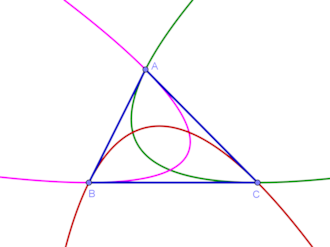
If you know the distance d to a satellite, you can compute a circle of points that passes through your location. That’s because you’re at the intersection of two spheres—the earth’s surface and a sphere of radius d centered on the satellite—and the intersection of two spheres is a circle. Said another way, one observation of a satellite determines a circle of possible locations.

If you know the distance to a second satellite as well, then you can find two circles that contain your location. The two circles intersect at two points, and you know that you’re at one of two possible positions. If you know your approximate position, you may be able to rule out one of the intersection points.

If you know the distance to three different satellites, now you know three circles that you’re standing on, and the third circle will only pass through one of the two points determined by the first two satellites. Now you know exactly where you are.

Knowing the distance to more satellites is even better. In theory additional observations are redundant but harmless. In practice, they let you partially cancel out inevitable measurement errors.

If you’re not on the earth’s surface, you’re still at the intersection of n spheres if you know the distance to n satellites. If you’re in an airplane, or on route to the moon, the same principles apply.

Errors and corrections

How do you know the distance to a satellite? The satellite can announce what time it is by its clock, then when you receive the announcement you compare it to the time by your clock. The difference between the two times tells you how long the radio signal traveled. Multiply by the speed of light and you have the distance.

However, your clock will probably not be exactly synchronized with the satellite clock. Observing a fourth satellite can fix the problem of your clock not being synchronized with the satellite clocks. But it doesn’t fix the more subtle problems of special relativity and general relativity. See this post by Shri Khalpada for an accessible discussion of the physics.

Numerical computation

Each distance measurement gives you an equation:

|| xsi || = di

where si is the location of the ith satellite and di is your distance to that satellite. If you square both sides of the equation, you have a quadratic equation. You have to solve a system of nonlinear equations, and yet there is a way to transform the problem into solving linear equations, i.e. using linear algebra. See this article for details.

Related posts

Finding a parabola through two points with given slopes

The Wikipedia article on modern triangle geometry has an image labeled “Artzt parabolas” with no explanation.

A quick search didn’t turn up anything about Artzt parabolas [1], but apparently the parabolas go through pairs of vertices with tangents parallel to the sides.

The general form of a conic section is

ax² + bxy + cy² + dx + ey + f = 0

and the constraint b² = 4ac means the conic will be a parabola.

We have 6 parameters, each determined only up to a scaling factor; you can multiply both sides by any non-zero constant and still have the same conic. So a general conic has 5 degrees of freedom, and the parabola condition b² = 4ac takes us down to 4. Specifying two points that the parabola passes through takes up 2 more degrees of freedom, and specifying the slopes takes up the last two. So it’s plausible that there is a unique solution to the problem.

There is indeed a solution, unique up to scaling the parameters. The following code finds parameters of a parabola that passes through (xi, yi) with slope mi for i = 1, 2.

def solve(x1, y1, m1, x2, y2, m2):
    
    Δx = x2 - x1
    Δy = y2 - y1
    λ = 4*(Δx*m1 - Δy)*(Δx*m2 - Δy)/(m1 - m2)**2
    k = x2*y1 - x1*y2

    a = Δy**2 + λ*m1*m2
    b = -2*Δx*Δy - λ*(m1 + m2)
    c = Δx**2 + λ
    d =  2*k*Δy + λ*(m1*y2 + m2*y1 - m1*m2*(x1 + x2))
    e = -2*k*Δx + λ*(m1*x1 + m2*x2 - y1 - y2)
    f = k**2 + λ*(m1*x1 - y1)*(m2*x2 - y2)

    return (a, b, c, d, e, f)

[1] The page said “Artz” when I first looked at it, but it has since been corrected to “Artzt”. Maybe I didn’t find anything because I was looking for the wrong spelling.

Random hexagon fractal

I recently ran across a post on X describing a process for creating a random fractal. First, pick a random point c inside a hexagon.

Then at each subsequent step, pick a random side of the hexagon and create the triangle formed by that side and c. Update c to be the center of the new triangle and plot c.

Note that you only choose a random point inside the hexagon once. After that you randomly choose sides.

Now there are many ways to define the center of a triangle. I assumed the original meant barycenter (centroid) when it said “center”, and apparently that was correct. I was able to create a similar figure.

But if you define center differently, you get a different image. For example, here’s what you get when you use the incenter, the center of the largest circle inside the triangle.

Related posts

Hyperbolic version of Napier’s mnemonic

I was looking through an old geometry book [1] and saw a hyperbolic analog of Napier’s mnemonic for spherical trigonometry. In hindsight of course there’s a hyperbolic analog: there’s a hyperbolic analog of everything. But I was surprised because I’d never thought of this before. I suppose the spherical version is famous because of its practical use in navigational calculations, while the hyperbolic analog is of more theoretical interest.

Napier’s mnemonic is a clever way to remember 10 equations in spherical trig. See the linked post for the meanings of the variables.

sin a = sin A sin c = tan b cot B
sin b = sin B sin c = tan a cot A
cos A = cos a sin B = tan b cot c
cos B = cos b sin A = tan a cot c
cos c = cot A cot B = cos a cos b

The hyperbolic analog replaces every circular function of ab, or c with its hyperbolic counterpart.

sinh a = sin A sinh c = tanh b cot B
sinh b = sin B sinh c = tanh a cot A
cos A = cosh a sin B = tanh b coth c
cos B = cosh b sin A = tanh a coth c
cosh c = cot A cot B = cosh a cosh b

[1] D. M. Y. Sommerville. The Elements of Non-Euclidean Geometry. 1919.

Visualizing orbital velocity

The shape of a planet’s orbit around a star is an ellipse. To put it another way, a plot of the position of a planet’s orbit over time forms an ellipse. What about the velocity? Is its plot also an ellipse? Surprisingly, a plot of the velocity forms a circle even if a plot of the position is an ellipse.

If an object is in a circular orbit, it’s velocity vector traces out a circle too, with the same center. If the object is in an elliptical orbit, it’s velocity vector still traces out a circle, but one with a different center. When the orbit is eccentric, the hodograph, the figure traced out by the velocity vector, is also eccentric, though the two uses of the word “eccentric” are slightly different.

The eccentricity e of an ellipse is the ratio c/a where c is the distance between the two foci and a is the semi-major axis. For a circle, c = 0 and so e = 0. The more elongated an ellipse is, the further apart the foci are relative to the axes and so the greater the eccentricity.

The plot of the orbit is eccentric in the sense that the two foci are distinct because the shape is an ellipse. The hodograph is eccentric in the sense that the circle is not centered at the origin.

The two kinds of eccentricity are related: the displacement of the center of the hodograph from the origin is proportional to the eccentricity of the ellipse.

Imagine the the orbit of a planet with its major axis along the x-axis and the coordinate of its star positive.  The hodograph is a circle shifted up by an amount proportional to the eccentricity of the orbit e. The top of the circle corresponds to perihelion, the point closest to the star, and the bottom corresponds to aphelion, the point furthest from the star. For more details, see the post Max and min orbital speed.

Solving spherical triangles

This post is a side quest in the series on navigating by the stars. It expands on a footnote in the previous post.

There are six pieces of information associated with a spherical triangle: three sides and three angles. I said in the previous post that given three out of these six quantities you could solve for the other three. Then I dropped a footnote saying sometimes the missing quantities are uniquely determined but sometimes there are two solutions and you need more data to uniquely determine a solution.

Todhunter’s textbook on spherical trig gives a thorough account of how to solve spherical triangles under all possible cases. The first edition of the book came out in 1859. A group of volunteers typeset the book in TeX. Project Gutenberg hosts the PDF version of the book and the TeX source.

I don’t want to duplicate Todhunter’s work here. Instead, I want to summarize when solutions are or are not unique, and make comparisons with plane triangles along the way.

SSS and AAA

The easiest cases to describe are all sides or all angles. Given three sides of a spherical triangle (SSS), you can solve for the angles, as with a plane triangle. Also, given three angles (AAA) you can solve for the remaining sides of a spherical triangle, unlike a plane triangle.

SAS and SSA

When you’re given two sides and an angle, there is a unique solution if the angle is between the two sides (SAS), but there may be two solutions if the angle is opposite one of the sides (SSA). This is the same for spherical and plane triangles.

There could be even more than two solutions in the spherical case. Consider a triangle with one vertex at the North Pole and two vertices on the equator. Two sides are specified, running from the pole to the equator, and the angles at the equator are specified—both are right angles—but the side of the triangle on the equator could be any length.

ASA and AAS

When you’re given two angles and a side, there is a unique solution if the side is common to the two angles (ASA).

If the side is opposite one of the angles (AAS), there may be two solutions to a spherical triangle, but only one solution to a plane triangle. This is because two angles uniquely determine the third angle in a plane triangle, but not in a spherical triangle.

The example above of a triangle with one vertex at the pole and two on the equator also shows that an AAS problem could have a continuum of solutions.

Summary

\begin{tabular}{|l|c|c|} \hline \textbf{Case} & \textbf{Plane} & \textbf{Spherical} \\ \hline SSS & 1 & 1 \\ SAS & 1 & 1 \\ SSA & 1 or 2 & 1 or 2 \\ AAS & 1 & 1 or 2 \\ ASA & 1 & 1 \\ AAA & $\infty$ & 1 \\ \hline \end{tabular}

Note that spherical triangles have a symmetry that plane triangles don’t: the spherical column above remains unchanged if you swap S’s and A’s. This is an example of duality in spherical geometry.

A triangle whose interior angles sum to zero

Spherical geometry

In spherical geometry, the interior angles of a triangle add up to more than π. And in fact you can determine the area of a spherical triangle by how much the angle sum exceeds π. On a sphere of radius 1, the area equals the triangle excess

Area = E = interior angle sum − π.

Small triangles have interior angle sum near π. But you could, for example, have a triangle with three right angles: put a vertex on the north pole and two vertices on the equator 90° longitude apart.

Hyperbolic geometry

In hyperbolic geometry, the sum of the interior angles of a triangle is always less than π. In a space with curvature −1, the area equals the triangle defect, the difference between π and the angle sum.

Area = D = π − interior angle sum.

Again small triangles have an interior angle sum near π. Both spherical and hyperbolic geometry are locally Euclidean.

The interior angle sum can be any value less than π, and so as the angle sum goes to 0, the triangle defect, and hence the area, goes to π. Since the minimum angle sum is 0, the maximum area of a triangle is π.

The figure below has interior angle sum 0 and area π in hyperbolic geometry.

Strictly speaking this is an improper triangle because the three hyperbolic lines (i.e. half circles) don’t intersect within the hyperbolic plane per se but at ideal points on the real axis. But you could come as close to this triangle as you like, staying within the hyperbolic plane.

Note that the radii of the (Euclidean) half circles doesn’t change the area. Any three semicircles that intersect on the real line as above make a triangle with the same area. Note also that the triangle has infinite perimeter but finite area.

Related posts

A circle in the hyperbolic plane

Let ℍ be the upper half plane, the set of complex real numbers with positive imaginary part. When we measure distances the way we’ve discussed in the last couple posts, the geometry of ℍ is hyperbolic.

What is a circle of radius r in ℍ? The same as a circle in any geometry: it’s the set of points a fixed distance r from a center. But when you draw a circle using one metric, it may look very different when viewed from the perspective of another metric.

Suppose we put on glasses that gave us a hyperbolic perspective on ℍ, draw a circle of radius r centered at i, then take off the hyperbolic glasses and put on Euclidean glasses. What would our drawing look like?

In the previous post we gave several equivalent expressions for the hyperbolic metric. We’ll use the first one here.

d(z_1, z_2) = 2\, \text{arcsinh}\left( \frac{|z_1 - z_2|}{2\, \sqrt{\Im z_1\, \Im z_2}} \right)

Here the Fraktur letter ℑ stands for imaginary part. So the set of points in a circle of radius r centered at i is

\{ x + iy \mid d(x + iy, i) = r \}

Divide the expression for d(xiyi) by 2, apply sinh, and square. This gives us

\sinh^2\left(\frac{r}{2}\right) = \frac{x^2 + (y-1)^2}{4y}

which is an equation for a Euclidean circle. If we multiply both sides by 4y and complete the square, we find that the center of the circle is (0, cosh(r)) and the radius is sinh(r).

Summary so far

So to recap, if we put on our hyperbolic glasses and draw a circle, then switch out these glasses for Euclidean glasses, the figure we drew again looks like a circle.

To put it another way, a hyperbolic viewer and a Euclidean viewer would agree that a circle has been draw. However, the two viewers would disagree where the center of the circle is located, and they would disagree on the radius.

Both would agree that the center is on the imaginary axis, but the hyperbolic viewer would say the imaginary part of the center is 1 and the Euclidean viewer would say it’s cosh(r). The hyperbolic observer would say the circle has radius r, but the Euclidean observer would say it has radius sinh(r).

Small circles

For small r, the hyperbolic and Euclidean viewpoints nearly agree because

cosh(r) = 1 + O(r²)

and

sinh(r) = r + O(r³)

Big circles

Note that if you asked a Euclidean observer to draw a circle of radius 100, centered at (0, 1), he would say that the circle will extend outside of the half plane. A hyperbolic observer would disagree. From his perspective, the real axis is infinitely far away and so he can draw a circle of any radius centered at any point and stay within the half plane.

Moving circles

Now what if we looked at circles centered somewhere else? The hyperbolic metric is invariant under Möbius transformations, and so in particular it is invariant under

zx0 + y0 z.

This takes a circle with hyperbolic center i to a circle centered at x0i y0 without changing the hyperbolic radius. The Euclidean center moves from cosh(r) to y0 cosh(r) and the radius changes from sinh(r) to y0 sinh(r).

Hyperbolic metric

One common model of the hyperbolic plane is the Poincaré upper half plane ℍ. This is the set of points in the complex plane with positive imaginary part. Straight lines are either vertical, a set of points with constant imaginary part, or arcs of circles centered on the real axis. The real axis is not part of ℍ. From the perspective of hyperbolic geometry these are ideal parts, infinitely far away, and not part of the plane itself.

We can define a metric on ℍ as follows. To find the distance between two points u and v, draw a line between the two points, and let a and b be the ideal points at the end of the line. By a line we mean a line as defined in the geometry of ℍ, what we would see from our Euclidean perspective as a half circle or a vertical line. Then the distance between u and v is defined as the absolute value of the log of the cross ratio (u, v; ab).

d(u, v) = |\log (u, v; a, b) | = \left| \log \frac{|a - u|\,|b - v|}{|a - v|\,|b - u|} \right|
Cross ratios are unchanged by Möbius transformations, and so Möbius transformations are isometries.

Another common model of hyperbolic geometry is the Poincaré disk. We can use the same metric on the Poincaré disk because the Möbius transformation

z \mapsto \frac{z - i}{z + i}

maps the upper half plane to the unit disk. This is very similar to how the Smith chart is created by mapping a grid in the right half plane to the unit disk.

Update: See the next post for four analytic expressions for the metric, direct formulas involving u and v but not the ideal points a and b.

Four generalizations of the Pythagorean theorem

Here are four theorems that generalize the Pythagorean theorem. Follow the links for more details regarding each equation.

1. Theorem by Apollonius for general triangles.

a^2 + b^2 = 2(m^2 + h^2)

2. Edsgar Dijkstra’s extension of the Pythagorean theorem for general triangles.

\text{sgn}(\alpha + \beta - \gamma) = \text{sgn}(a^2 + b^2 - c^2)

3. A generalization of the Pythagorean theorem to tetrahedra.

V_0^2 = \sum_{i=1}^n V_i^2

4. A unified Pythagorean theorem that covers spherical, plane, and hyperbolic geometry.

A(c) = A(a) + A(b) - \kappa \frac{A(a) \, A(b)}{2\pi}