A couple days ago I analyzed the observation that repeatedly pressing the cosine key on a calculator leads to a fixed point. After about 90 iterations the number no longer changes. This post will analyze the same phenomenon a different way.
Interval arithmetic
Interval arithmetic is a way to get exact results of a sort from floating point arithmetic.
Suppose you start with a number x that cannot be represented exactly as a floating point number, and you want to compute f(x) for some function f. You can’t represent x exactly, but unless x is too large you can represent a pair of numbers a and b such that x is certainly in the interval [a, b]. Then f(x) is in the set f( [a, b] ).
Maybe you can represent f( [a, b] ) exactly. If not, you can enlarge the interval a bit to exactly represent an interval that contains f(x). After applying several calculations, you have an interval, hopefully one that’s not too big, containing the exact result.
(I said above that interval arithmetic gives you exact results of a sort because even though you don’t generally get an exact number at the end, you do get an exact interval containing the result.)
Cosine iteration
In this post we will use interval arithmetic, not to compensate for the limitations of computer arithmetic, but to illustrate the convergence of iterated cosines.
The cosine of any real number lies in the interval [−1, 1]. To put it another way,
cos( [−∞, ∞] ) = [−1, 1].
Because cosine is an even function,
cos( [−1, 1] ) = cos( [0, 1] )
and so we can limit our attention to the interval [0, 1].
Now the cosine is a monotone decreasing function from 0 to π, and so it’s monotone on [0, 1]. For any two points with 0 ≤ a ≤ b ≤ π we have
cos( [a, b] ) = [cos(b), cos(a)].
Note that the order of a and b reverses on the right hand side of the equation because cosine is decreasing. When we apply cosine again we get back the original order.
cos(cos( [a, b] )) = [cos(cos(a)), cos(cos(b))].
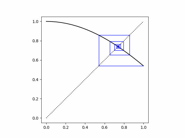
Incidentally, this flip-flop explains why the cobweb plot from the previous post looks like a spiral rather than a staircase.
Now define a0 = 0, b0 = 1, and
[an+1, bn+1] = cos( [an, bn] ) = [cos(bn), cos(an)].
We could implement this in Python with a pair of mutually recursive functions.
    a = lambda n: 0 if n == 0 else cos(b(n-1))
    b = lambda n: 1 if n == 0 else cos(a(n-1))
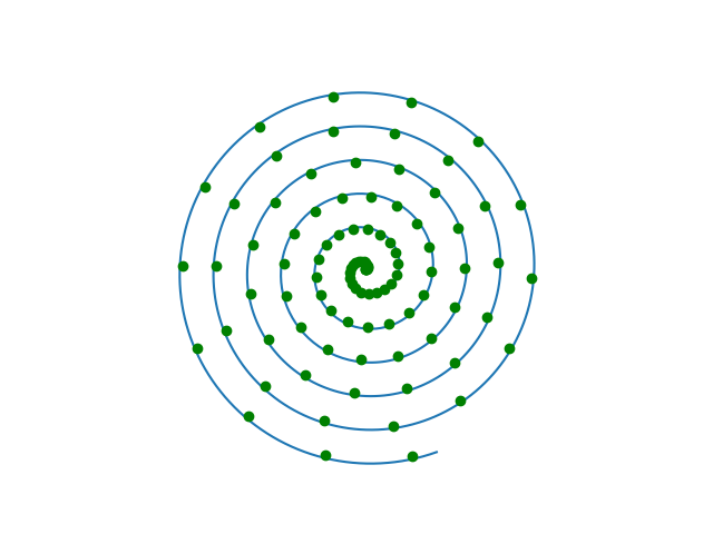
Here’s a plot of the image of [0, 1] after n iterations.
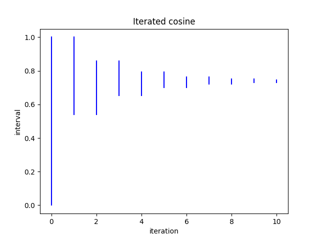
Note that odd iterations increase the lower bound and even iterations decrease the upper bound.
Numerical interval arithmetic
This post introduced interval arithmetic as a numerical technique, then proceeded to do pure math. Now let’s think about computing again.
The image of [0, 1] under cosine is [cos(1), cos(0)] = [cos(1), 1]. A computer can represent 1 exactly but not cos(1). Suppose we compute
cos(1) = 0.5403023058681398
and assume each digit in the result is correct. Maybe the exact value of cos(1) was slightly smaller and was rounded to this value, but we know for sure that
cos( [0, 1] ) ⊂ [0.5403023058681397, 1]
So in this case we don’t know the image of [0, 1], but we know an interval that contains the image, hence the subset symbol.
We could iterate this process, next computing an interval that contains
cos( [0.5403023058681397, 1] )
and so forth. At each step we would round the left endpoint down to the nearest representable lower bound and round the right endpoint up to the nearest representable upper bound. In practice we’d be concerned with machine representable numbers rather than decimal representable numbers, but the principle is the same.
The potential pitfall of interval arithmetic in practice is that intervals may grow so large that the final result is not useful. But that’s not the case here. The rounding error at each step is tiny, and contraction maps reduce errors at each step rather than magnifying them. In a more complicated calculation, we might have to resort to lose estimates and not have such tight intervals at each step.
Related posts