The hardest logarithm to compute

Suppose you want to compute the natural logarithms of every floating point number, correctly truncated to a floating point result. Here by floating point number we mean an IEEE standard 64-bit float, what C calls a double. Which logarithm is hardest to compute?

We’ll get to the hardest logarithm shortly, but we’ll first start with a warm up problem. Suppose you needed to compute the first digit of a number z. You know that z equals 2 + ε where ε is either 10−100 or −10−100. If ε is positive, you should return 2. If ε is negative, you should return 1. You know z to very high precision a priori, but to return the first digit correctly, you need to compute z to 100 decimal places.

In this post we’re truncating floating point numbers, i.e. rounding down, but similar considerations apply when rounding to nearest. For example, if you wanted to compute 0.5 + ε rounded to the nearest integer.

In general, it may not be possible to know how accurately you need to compute a value in order to round it correctly. William Kahan called this the table maker’s dilemma.

Worst case for logarithm

Lefèvre and Muller [1] found that the floating point number whose logarithm is hardest to compute is

x = 1.0110001010101000100001100001001101100010100110110110 × 2678

where the fractional part is written in binary. The log of x, again written in binary, is

111010110.0100011110011110101110100111110010010111000100000000000000000000000000000000000000000000000000000000000000000111 …

The first 53 significant bits, all the bits a floating point number can represent [2], are followed by 65 zeros. We have to compute the log with a precision of more than 118 bits in order to know whether the last bit of the fraction part of the float representation should be a 0 or a 1. Usually you don’t need nearly that much precision, but this is the worst case.

Mathematica code

Here is Mathematica code to verify the result above. I don’t know how to give Mathematica floating point numbers in binary, but I know how to give it integers, so I’ll multiply the fraction part by 252 and take 52 from the exponent.

n = FromDigits[
  "10110001010101000100001100001001101100010100110110110", 2]
x = n  2^(678 - 52)
BaseForm[N[Log[x], 40], 2]

This computes the log of x to 40 significant decimal figures, between 132 and 133 bits, and gives the result above.

Related posts

A few days ago I wrote about another example by Jean-Michel Muller: A floating point oddity.

William Kahan also came up recently in my post on summing an array of floating point numbers.

***

[1] Vincent Lefèvre, Jean-Michel Muller. Worst Cases for Correct Rounding of the Elementary Functions in Double Precision. November 2000. Research Report 2000-35. Available here.

[2] There are 52 bits in the faction of an IEEE double. The first bit of a fraction is 1, unless a number is subnormal, so the first bit is left implicit, squeezing out one extra bit of precision. That is, storing 52 bits gives us 53 bits of precision.

Summing an array of floating point numbers

Adding up an array of numbers is simple: just loop over the array, adding each element to an accumulator.

Usually that’s good enough, but sometimes you need more precision, either because your application need a high-precision answer, or because your problem is poorly conditioned and you need a moderate-precision answer [1].

There are many algorithms for summing an array, which may be surprising if you haven’t thought about this before. This post will look at Kahan’s algorithm, one of the first non-obvious algorithms for summing a list of floating point numbers.

We will sum a list of numbers a couple ways using C’s float type, a 32-bit floating point number. Some might object that this is artificial. Does anyone use floats any more? Didn’t moving from float to double get rid of all our precision problems? No and no.

In fact, the use of 32-bit float types is on the rise. Moving data in an out of memory is now the bottleneck, not arithmetic operations per se, and float lets you pack more data into a giving volume of memory. Not only that, there is growing interest in floating point types even smaller than 32-bit floats. See the following posts for examples:

And while sometimes you need less precision than 32 bits, sometimes you need more precision than 64 bits. See, for example, this post.

Now for some code. Here is the obvious way to sum an array in C:

    float naive(float x[], int N) {
        float s = 0.0;
        for (int i = 0; i < N; i++) {
            s += x[i];
        }
        return s;
    }

Kahan’s algorithm is not much more complicated, but it looks a little mysterious and provides more accuracy.

    float kahan(float x[], int N) {
        float s = x[0];
        float c = 0.0;
        for (int i = 1; i < N; i++) {
            float y = x[i] - c;
            float t = s + y;
            c = (t - s) - y;
            s = t;
        }
        return s;
    }

Now to compare the accuracy of these two methods, we’ll use a third method that uses a 64-bit accumulator. We will assume its value is accurate to at least 32 bits and use it as our exact result.

    double dsum(float x[], int N) {
        double s = 0.0;
        for (int i = 0; i < N; i++) {
            s += x[i];
        }
        return s;
    }

For our test problem, we’ll use the reciprocals of the first 100,000 positive integers rounded to 32 bits as our input. This problem was taken from [2].

    #include <stdio.h>
    int main() {
        int N = 100000;
        float x[N];
        for (int i = 1; i <= N; i++)
            x[i-1] = 1.0/i;
  
        printf("%.15g\n", naive(x, N));
        printf("%.15g\n", kahan(x, N));  
        printf("%.15g\n", dsum(x, N));
    }

This produces the following output.

    12.0908508300781
    12.0901460647583
    12.0901461953972

The naive method is correct to 6 significant figures while Kahan’s method is correct to 9 significant figures. The error in the former is 5394 times larger. In this example, Kahan’s method is as accurate as possible using 32-bit numbers.

Note that in our example we were not exactly trying to find the Nth harmonic number, the sum of the reciprocals of the first N positive numbers. Instead, we were using these integer reciprocals rounded to 32 bits as our input. Think of them as just data. The data happened to be produced by computing reciprocals and rounding the result to 32-bit floating point accuracy.

But what if we did want to compute the 100,000th harmonic number? There are methods for computing harmonic numbers directly, as described here.

Related posts

[1] The condition number of a problem is basically a measure of how much floating point errors are multiplied in the process of computing a result. A well-conditioned problem has a small condition number, and a ill-conditioned problem has a large condition number. With ill-conditioned problems, you may have to use extra precision in your intermediate calculations to get a result that’s accurate to ordinary precision.

[2] Handbook of Floating-Point Arithmetic by Jen-Michel Muller et al.

Arbitrary precision is not a panacea

Having access to arbitrary precision arithmetic does not necessarily make numerical calculation difficulties go away. You still need to know what you’re doing.

Before you extend precision, you have to know how far to extend it. If you don’t extend it enough, your answers won’t be accurate enough. If you extend it too far, you waste resources. Maybe you’re OK wasting resources, so you extend precision more than necessary. But how far is more than necessary?

As an example, consider the problem of finding values of n such that tan(n) > n discussed a couple days ago. After writing that post, someone pointed out that these values of n are one of the sequences on OEIS. One of the values on the OEIS site is

k = 1428599129020608582548671.

Let’s verify that tan(k) > k. We’ll use our old friend bc because it supports arbitrary precision. Our k is a 25-digit number, so lets tell bc we want to work with 30 decimal places to give ourselves a little room. (bc automatically gives you a little more room than you ask for, but we’ll ask for even more.)

bc doesn’t have a tangent function, but it does have s() for sine and c() for cosine, so we’ll compute tangent as sine over cosine.

    $ bc -l
    scale = 30
    k = 1428599129020608582548671
    s(k)/c(k) - k

We expect this to return a positive value, but instead it returns

-1428599362980017942210629.31…

So is OEIS wrong? Or is bc ignoring our scale value? It turns out neither is true.

You can’t directly compute the tangent of a large number. You use range reduction to reduce it to the problem of computing the tangent of a small angle where your algorithms will work. Since tangent has period π, we reduce k mod π by computing k − ⌊k/π⌋π. That is, we subtract off as many multiples of π as we can until we get a number between 0 and π. Going back to bc, we compute

    pi = 4*a(1)
    k/pi

This returns

    454737226160812402842656.500000507033221370444866152761

and so we compute the tangent of

    t = 0.500000507033221370444866152761*pi
      = 1.570797919686740002588270178941

Since t is slightly larger than π/2, the tangent will be negative. We can’t have tan(t) greater than k because tan(t) isn’t even greater than 0. So where did things break down?

The calculation of pi was accurate to 30 significant figures, and the calculation of k/pi was accurate to 30 significant figures, given our value of pi. So far has performed as promised.

The computed value of k/pi is correct to 29 significant figures, 23 before the decimal place and 6 after. So when we take the fractional part, we only have six significant figures, and that’s not enough. That’s where things go wrong. We get a value ⌊k/π⌋ that’s greater than 0.5 in the seventh decimal place while the exact value is less than 0.5 in the 25th decimal place. We needed 25 − 6 = 19 more significant figures.

This is the core difficulty with floating point calculation: subtracting nearly equal numbers loses precision. If two numbers agree to m decimal places, you can expect to lose m significant figures in the subtraction. The error in the subtraction will be small relative to the inputs, but not small relative to the result.

Notice that we computed k/pi to 29 significant figures, and given that output we computed the fractional part exactly. We accurately computed ⌊k/π⌋π, but lost precision when we computed we subtracted that value from k.

Our error in computing k − ⌊k/π⌋π was small relative to k, but not relative to the final result. Our k is on the order of 1025, and the error in our subtraction is on the order of 10−7, but the result is on the order of 1. There’s no bug in bc. It carried out every calculation to the advertised accuracy, but it didn’t have enough working precision to produce the result we needed.

Related posts

Higher order Newton-like methods for root finding

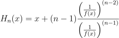
There are variations on Newton’s root finding method that use higher derivatives and converge faster. Alston Householder developed a sequence of such methods of the form

H_n(x) = x + (n-1) \frac{\left( \frac{1}{f(x)}\right)^{(n-2)}}{\left( \frac{1}{f(x)}\right)^{(n-1)}}

where the superscripts in parentheses indicate derivatives. When n = 2, Householder’s method reduces to Newton’s method.

Once Newton’s method is close enough to a root, the error is squared at each iteration. Said another way, the number of correct decimal places roughly doubles. With the Householder method of order n, the number of correct decimal places roughly increases by a factor of n.

The Householder method Hn can be written as a rational function of f and its derivatives up to order n − 1, though the formulas are complicated.

Maybe it’s time for Householder’s methods to be more widely used: with automatic differentiation [1], the complexity of computing higher order derivatives is not the drawback it was when these computations were done solely by hand.

Demonstration

We’ll illustrate the convergence of the Householder methods by finding roots of the quintic polynomial

f(x) = x5 + ax + b.

I used Mathematica to calculate expressions for the Householder methods and export the results as code. Mathematica does not have a function to export Python code, but it does have a function CForm to export expressions as C code. I started to use this, converting exponents from C to Python form with search and replace. Then I tried using FortranForm instead, and that was much easier because Fortran and Python both represent powers with a ** operator.

def f(x, a, b):
    return x**5 + a*x + b

def H2(x, a, b):
    return x - (b + a*x + x**5)/(a + 5*x**4)
    
def H3(x, a, b):
    num = (a + 5*x**4)*(b + a*x + x**5)
    den = a**2 - 10*b*x**3 + 15*x**8
    return x - num/den

def H4(x, a, b):
    num = (b + a*x + x**5)*(-a**2 + 10*b*x**3 - 15*x**8)
    den = a**3 + 10*b**2*x**2 + 5*a**2*x**4 - 80*b*x**7 - 25*a*x**8 + 35*x**12
    return x + num/den

To set values of a and b, I arbitrarily chose a = 2 and solved for b so that π is a root. That way we have a known value of the root for comparison. I used x = 4 as my starting guess at the root.

I first used −log10|x − π| to measure the number of correct decimals. That didn’t quite work because the method would converge exactly (to the limits of machine precision) which led to taking the log of zero. So I modified my accuracy function to the following.

def decimals(x):
    d = abs(x - pi)
    if d != 0:
        return( round(-log10(d),2) )
    else:
        return "inf"

Then I tested each of the Householder methods with the following.

epsilon = 1e-14
for H in [H2, H3, H4]:
    x = 4
    for i in range(1, 10):
        if abs(f(x,a,b)) > epsilon:
            x = H(x,a,b)
            print(i, x, decimals(x))

Here are the results in tabular form. I replaced all the decimals after the first incorrect decimal with underscores to make it easier to see the convergence.

|---+-------------------+--------|
| i |                 x | digits |
|---+-------------------+--------|
| 1 | 3.4______________ |   0.53 |
| 2 | 3.18_____________ |   1.33 |
| 3 | 3.142____________ |   2.87 |
| 4 | 3.141593_________ |   5.93 |
| 5 | 3.141592653590___ |  12.07 |
| 6 | 3.141592653589793 |    inf |
|---+-------------------+--------|
| 1 | 3.2______________ |   1.11 |
| 2 | 3.1416___________ |   4.03 |
| 3 | 3.1415926535899__ |  12.79 |
| 4 | 3.141592653589793 |    inf |
|---+-------------------+--------|
| 1 | 3.15_____________ |   1.84 |
| 2 | 3.141592654______ |   8.85 |
| 3 | 3.141592653589793 |    inf |
|---+-------------------+--------|

Note that, as promised, the number of correct decimal places for Hn increases by roughly a factor of n with each iteration.

Update: See this post where the symbolic calculations are done in SymPy rather than Mathematica. Everything stays in Python, and there’s no need to edit the code for the Householder methods.

Related posts

[1] Note that in this post I used Mathematica to do symbolic differentiation, not automatic differentiation. Automatic differentiation differs from both symbolic and numerical differentiation. See an explanation here.

Euler’s method for accelerating an alternating series

The most direct way of computing the sum of an alternating series, simply computing the partial sums in the terms get small enough, may not be the most efficient. Euler figured this out in the 18th century.

For our demo we’ll evaluate the Struve function defined by the series

H_\nu(z) = (z/2)^{\nu + 1} \sum_{k=0}^\infty (-1)^k \frac{(z/2)^{2k}}{\Gamma\left(k + 3/2\right ) \, \Gamma\left(k + \nu + 3/2 \right )}

Note that the terms in the series are relatively expensive to evaluate since each requires evaluating a gamma function. Euler’s acceleration method will be inexpensive relative to computing the terms it takes as input.

Here’s what we get by evaluating the first partial sums for H1.2(3.4):

    2.34748
    0.67236
    1.19572
    1.10378
    1.11414
    1.11332

So if we were to stop here, we’d report 1.11332 as the value of H1.2(3.4).

Next let’s see what we’d get using Euler’s transformation for alternating series. I’ll full precision in my calculations internally but only displaying four digits to save horizontal space that we’ll need shortly.

    2.3474 1.5099 
    0.6723 0.9340 
    1.1957 1.1497 
    1.1037 1.1089  
    1.1141 1.1137
    1.1133 

Now we repeat the process again, taking averages of consecutive terms in each column to produce the next column.

    2.3474 1.5099 1.2219 1.1319 1.1087 1.1058
    0.6723 0.9340 1.0418 1.0856 1.1029 
    1.1957 1.1497 1.1293 1.1203 
    1.1037 1.1089 1.1113 
    1.1141 1.1137 
    1.1133 

The terms across the top are the Euler approximations to the series. The final term 1.1058 is the Euler approximation based on all six terms. And it is worse than what we get from simply taking partial sums!

The exact value is 1.11337… and so the sixth partial sum was accurate to four decimal places, but our clever method was only good to one decimal place.

What went wrong?! Euler’s method is designed to speed up the convergence of slowly converging alternating series. But our series converges pretty quickly because it has two terms in the denominator that grow like factorials. When you apply acceleration when you don’t need to, you can make things worse. Since our series was already converging quickly, we would have done better to use Aitken acceleration, the topic of the next post.

But Euler’s method works well when it’s needed. For example, let’s look at the slowly converging series

π = 4 − 4/3 + 4/5 − 4/7 + 4/9 − …

Then we get the following array.

    4.0000 3.3333 3.200o 3.1619 3.1492 3.1445
    2.6666 3.0666 3.1238 3.1365 3.1399 
    3.4666 3.1809 3.1492 3.1434
    2.8952 3.1174 3.1376 
    3.3396 3.1578
    2.9760

The sequence of partial sums is along the left side, and the series of Euler terms is across the top row. Neither gives a great approximation to π, but the approximation error using Euler’s acceleration method is 57 times smaller than simply using the partial sums.

Related series posts

Taking the derivative of a muscle car

I’ve been getting a lot of spam lately saying my website does not rank well on “certain keywords.” This is of course true: no website ranks well for every keyword.

I was joking about this on Twitter, saying that my site does not rank well for women’s shoes, muscle cars, or snails because I don’t write about these topics. J. D. Long replied saying I should write more about muscle cars.

My first thought was to do an example drawing a Shelby Cobra with cubic splines. This would not be such an artificial example. Mathematical splines are named after physical splines, devices that have been used in designing, among other things, cars.

Instead, I downloaded an image of a Shelby Cobra from Wikipedia

Original image

and played with it in Mathematica. Specifically, I applied a Sobel filter which you can think of as a kind of derivative, looking for edges, places where the pixel values have a sharp change.

Sobol filtered image

Here’s the same image with the colors reversed.

Cobra image reversed

Here’s the Mathematica code to do the edge detection.

    cobra = Import["c:/users/mail/desktop/cobra.jpg"]
    ImageConvolve[cobra, {{-1, 0, 1}, {-2, 0, 2}, {-1, 0, 1}}]

Computing SVD and pseudoinverse

In a nutshell, given the singular decomposition of a matrix A,

A = U \Sigma V^*

the Moore-Penrose pseudoinverse is given by

A^+ = V \Sigma^+ U^*.

This post will explain what the terms above mean, and how to compute them in Python and in Mathematica.

Singular Value Decomposition (SVD)

The singular value decomposition of a matrix is a sort of change of coordinates that makes the matrix simple, a generalization of diagonalization.

Matrix diagonalization

If a square matrix A is diagonalizable, then there is a matrix P such that

A = P D P^{-1}

where the matrix D is diagonal. You could think of P as a change of coordinates that makes the action of A as simple as possible. The elements on the diagonal of D are the eigenvalues of A and the columns of P are the corresponding eigenvectors.

Unfortunately not all matrices can be diagonalized. Singular value decomposition is a way to do something like diagonalization for any matrix, even non-square matrices.

Generalization to SVD

Singular value decomposition generalizes diagonalization. The matrix Σ in SVD is analogous to D in diagonalization. Σ is diagonal, though it may not be square. The matrices on either side of Σ are analogous to the matrix P in diagonalization, though now there are two different matrices, and they are not necessarily inverses of each other. The matrices U and V are square, but not necessarily of the same dimension.

The elements along the diagonal of Σ are not necessarily eigenvalues but singular values, which are a generalization of eigenvalues. Similarly the columns of U and V are not necessarily eigenvectors but left singular vectors and right singular vectors respectively.

The star superscript indicates conjugate transpose. If a matrix has all real components, then the conjugate transpose is just the transpose. But if the matrix has complex entries, you take the conjugate and transpose each entry.

The matrices U and V are unitary. A matrix M is unitary if its inverse is its conjugate transpose, i.e. M* M = MM* = I.

Pseudoinverse and SVD

The (Moore-Penrose) pseudoinverse of a matrix generalizes the notion of an inverse, somewhat like the way SVD generalized diagonalization. Not every matrix has an inverse, but every matrix has a pseudoinverse, even non-square matrices.

Computing the pseudoinverse from the SVD is simple.

If

A = U \Sigma V^*

then

A^+ = V \Sigma^+ U^*

where Σ+ is formed from Σ by taking the reciprocal of all the non-zero elements, leaving all the zeros alone, and making the matrix the right shape: if Σ is an m by n matrix, then Σ+ must be an n by m matrix.

We’ll give examples below in Mathematica and Python.

Computing SVD in Mathematica

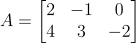
Let’s start with the matrix A below.

A = \begin{bmatrix} 2 & -1 & 0 \\ 4 & 3 & -2 \end{bmatrix}

We can find the SVD of A with the following Mathematica commands.

    A = {{2, -1, 0}, {4, 3, -2}}
    {U, S, V} = SingularValueDecomposition[A]

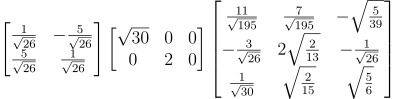
From this we learn that the singular value decomposition of A is

\begin{bmatrix} \frac{1}{\sqrt{26}} & -\frac{5}{\sqrt{26}} \\ \frac{5}{\sqrt{26}} & \frac{1}{\sqrt{26}} \\ \end{bmatrix} \begin{bmatrix} \sqrt{30} & 0 & 0 \\ 0 & 2 & 0 \end{bmatrix} \begin{bmatrix} \frac{11}{\sqrt{195}} & \frac{7}{\sqrt{195}} & -\sqrt{\frac{5}{39}} \\ -\frac{3}{\sqrt{26}} & 2 \sqrt{\frac{2}{13}} & -\frac{1}{\sqrt{26}} \\ \frac{1}{\sqrt{30}} & \sqrt{\frac{2}{15}} & \sqrt{\frac{5}{6}} \end{bmatrix}

Note that the last matrix is not V but the transpose of V. Mathematica returns V itself, not its transpose.

If we multiply the matrices back together we can verify that we get A back.

    U . S. Transpose[V]

This returns

    {{2, -1, 0}, {4, 3, -2}}

as we’d expect.

Computing pseudoinverse in Mathematica

The Mathematica command for computing the pseudoinverse is simply PseudoInverse. (The best thing about Mathematica is it’s consistent, predictable naming.)

    PseudoInverse[A]

This returns

    {{19/60, 1/12}, {-(11/30), 1/6}, {1/12, -(1/12)}}

And we can confirm that computing the pseudoinverse via the SVD

    Sp = {{1/Sqrt[30], 0}, {0, 1/2}, {0, 0}}
    V . Sp . Transpose[U]

gives the same result.

Computing SVD in Python

Next we compute the singular value decomposition in Python (NumPy).

    >>> a = np.matrix([[2, -1, 0],[4,3,-2]])
    >>> u, s, vt = np.linalg.svd(a, full_matrices=True)

Note that np.linalg.svd returns the transpose of V, not the V in the definition of singular value decomposition.

Also, the object s is not the diagonal matrix Σ but a vector containing only the diagonal elements, i.e. just the singular values. This can save a lot of space if the matrix is large. The NumPy method svd has other efficiency-related options that I won’t go into here.

We can verify that the SVD is correct by turning s back into a matrix and multiply the components together.

    >>> ss = np.matrix([[s[0], 0, 0], [0, s[1], 0]])
    >>> u*ss*vt

This returns the matrix A, within floating point accuracy. Since Python is doing floating point computations, not symbolic calculation like Mathematica, the zero in A turns into -3.8e-16.

Note that the singular value decompositions as computed by Mathematica and Python differ in a few signs here and there; the SVD is not unique.

Computing pseudoinverse in Python

The pseudoinverse can be computed in NumPy with np.linalg.pinv.

    >>> np.linalg.pinv(a)
    matrix([[ 0.31666667,  0.08333333],
            [-0.36666667,  0.16666667],
            [ 0.08333333, -0.08333333]])

This returns the same result as Mathematica above, up to floating point precision.

More linear algebra posts

Tridiagonal systems, determinants, and natural cubic splines

Tridiagonal matrices

A tridiagonal matrix is a matrix that has nonzero entries only on the main diagonal and on the adjacent off-diagonals. This special structure comes up frequently in applications. For example, the finite difference numerical solution to the heat equation leads to a tridiagonal system. Another application, the one we’ll look at in detail here, is natural cubic splines. And we’ll mention an interesting result with Fibonacci numbers in passing.

Because these matrices have a special structure, the corresponding linear systems are quick and easy to solve. Also, we can find a simple recurrence relation for their determinants.

Determinants

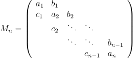
Let’s label the component of a tridiagonal matrix as below

M_n = \left( \begin{array}{lllll} a_1 & b_1 & & & \\ c_1 & a_2 & b_2 & & \\ & c_2 & \ddots & \ddots & \\ & & \ddots & \ddots & b_{n-1} \\ & & & c_{n-1} & a_n \\ \end{array} \right)

where every component not shown is implicitly zero. We can expand the determinant of the matrix above using minors along the last row. This gives a recursive expression for the determinant

d_n = a_n d_{n-1} - c_{n-1} b_{n-1} d_{n-2}

with initial conditions d0 = 1 and d−1 = 0.

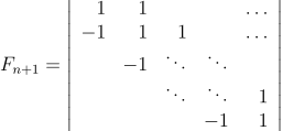
Note that if all the a‘s and b‘s are 1 and all the c‘s are −1, then you get the recurrence relation that defines the Fibonacci numbers. That is, the Fibonacci numbers are given by the determinant

F_{n+1} = \left| \begin{array}{rrrrr} 1 & 1 & & & \ldots \\ -1 & 1 & 1 & & \ldots \\ & -1 & \ddots & \ddots & \\ & & \ddots & \ddots & 1 \\ & & & -1 & 1 \\ \end{array} \right|

Natural cubic splines

A cubic spline interpolates a set of data points with piecewise cubic polynomials. There’s a (potentially) different cubic polynomial over each interval between input values, all fitted together so that the resulting function, its derivative, and its second derivative are all continuous.

Suppose you have input points, called knots in this context, t0, t1, … tn and output values y0, y1, … yn. For the spline to interpolate the data, its value at ti must be yi.

A cubic spline then is a set of n cubic polynomials, one for each interval [ti, ti+1]. A cubic polynomial has four coefficients, so we have 4n coefficients in total. At each interior knot, t1 through tn−1, we have four constraints. Both polynomials that meet at ti must take on the value yi at that point, and the two polynomials must have the same first and second derivative at that point. That gives us 4(n − 1) equations. The value of the first polynomial is specified on the left end at t0 the value of the last polynomial is specified at the right end at tn. This gives us 4n − 2 equations in total.

We need two more equations. A clamped cubic spline specifies the derivatives at each end point. The natural cubic spline specifies instead that the second derivatives at each end are zero. What is natural about a natural cubic spline? In a certain sense it is the smoothest curve interpolating the specified points. With these boundary conditions we now have as many constraints as degrees of freedom.

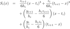
So how would we go about finding the coefficients of each polynomial? Our task will be much easier if we parameterize the polynomials cleverly to start with. Instead of powers of x, we want powers of (xti) and (ti+1x) because these expressions are 0 on different ends of the interval [ti, ti+1]. It turns out we parameterize the spline over the ith interval as

\begin{eqnarray*} S_i(x) &=& \frac{z_{i+1}}{6h_i}(x-t_i)^3 + \frac{z_i}{6h_i}(t_{i+1} - x)^3 \\ && + \left(\frac{y_{i+1}}{h_i} - \frac{h_iz_{i+1}}{6}\right) (x - t_i) \\ && + \left(\frac{y_{i }}{h_i} - \frac{h_iz_i }{6}\right) (t_{i+1} - x) \end{eqnarray*}

where hi = ti+1ti, the length of the ith interval.

This may seem unmotivated, and no doubt it is cleaner than the first thing someone probably tried, but it’s the kind of thing you’re lead to when you try to make the derivation work out smoothly.

The basic form is  powers of (xti) and (ti+1x), each to the first and third powers, for reasons given above. Why the 6’s in the denominators? They’re not strictly necessary, but they cancel out when we take second derivatives. Let’s look at the second derivative.

S_i''(x) = \frac{z_{i+1}(x - t_i)}{h_i} - \frac{z_{i}(t_{i+1} - x)}{h_i}

Note how when we stick in ti the first term is zero and the second is zi, and when we stick in ti+1 the first term is zi+1 and the second is zero.

We can now write down the system of equations for the z‘s. We have z0 = zn from the natural cubic spline condition, and for 1 ≤ in − 1 we have

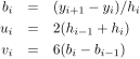
h_{i-1}z_{i-1} + u_i z_i + h_i z_{i+1} = v_i

where

\begin{eqnarray*}b_i &=& (y_{i+1} - y_i)/h_i \\ u_i &=& 2(h_{i-1} + h_i) \\ v_i &=& 6(b_i - b_{i-1}) \end{eqnarray*}
Note that this is a tridiagonal system because the ith equation only involves z‘s with subscripts i − 1, i, and i + 1.

Because of its tridiagonal structure, these equations can be solved simply and efficiently, much more efficiently than a general system of equations.

Related math posts

The quadratic formula and low-precision arithmetic

What could be interesting about the lowly quadratic formula? It’s a formula after all. You just stick numbers into it.

Well, there’s an interesting wrinkle. When the linear coefficient b is large relative to the other coefficients, the quadratic formula can give wrong results when implemented in floating point arithmetic.

Quadratic formula and loss of precision

The quadratic formula says that the roots of

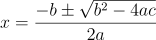
ax^2 + bx + c = 0

are given by

x = \frac{-b \pm \sqrt{b^2 - 4ac}}{2a}

That’s true, but let’s see what happens when we have ac = 1 and b = 108.

    from math import sqrt

    def quadratic(a, b, c):
        r = sqrt(b**2 - 4*a*c)
        return ((-b + r)/(2*a), (-b -r)/(2*a))

    print( quadratic(1, 1e8, 1) )

This returns

    (-7.450580596923828e-09, -100000000.0)

The first root is wrong by about 25%, though the second one is correct.

What happened? The quadratic equation violated the cardinal rule of numerical analysis: avoid subtracting nearly equal numbers. The more similar two numbers are, the more precision you can lose from subtracting them. In this case √(b² – 4ac) is very nearly equal to b.

If we ask Python to evaluate

    1e8 - sqrt(1e16-4)

we get 1.49e-8 when the correct answer would be 2.0e-8.

Improving precision for quadratic formula

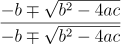
The way to fix the problem is to rationalize the numerator of the quadratic formula by multiplying by 1 in the form

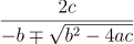
\frac{-b \mp \sqrt{b^2 - 4ac}}{-b \mp \sqrt{b^2 - 4ac}}

(The symbol ∓ is much less common than ±. It just means that if you take the + sign in the quadratic formula, take the − sign above, and vice versa.)

When we multiply by the expression above and simplify we get

\frac{2c}{-b \mp \sqrt{b^2 - 4ac}}

Let’s code this up in Python and try it out.

    def quadratic2(a, b, c):
        r = sqrt(b**2 - 4*a*c)
        return (2*c/(-b - r), 2*c/(-b+r))

    print( quadratic2(1, 1e8, 1) )

This returns

    (-1e-08, -134217728.0)

So is our new quadratic equation better? It gives the right answer for the first root, exact to within machine precision. But now the second root is wrong by 34%. Why is the second root wrong? Same reason as before: we subtracted two nearly equal numbers!

The familiar version of the quadratic formula computes the larger root correctly, and the new version computes the smaller root correctly. Neither version is better overall. We’d be no better off or worse off always using the new quadratic formula than the old one. Each one is better when it avoids subtracting nearly equal numbers.

The solution is to use both quadratic formulas, using the appropriate one for the root you’re trying to calculate.

Low precision arithmetic

Is this a practical concern? Yes, and here’s why: Everything old is new again.

The possible inaccuracy in the quadratic formula was serious before double precision (64-bit floating point) arithmetic became common. And back in the day, engineers were more likely to be familiar with the alternate form of the quadratic formula. You can still run into quadratic equations that give you trouble even in double precision arithmetic, like the example above, but it’s less likely to be a problem when you have more bits at your disposal.

Now we’re interested in low-precision arithmetic again. CPUs have gotten much faster, but moving bits around in memory has not. Relative to CPU speed, memory manipulation has gotten slower. That means we need to be more concerned with memory management and less concerned about floating point speed.

Not only is memory juggling slower relative to CPU, it also takes more energy. According to Gustafson, reading 64 bits from DRAM requires 65 times as much energy as doing a floating point combined multiply-add because it takes place off-chip. The table below, from page 6 of Gustafson’s book, gives the details. Using lower precision floating point saves energy because more numbers can be read in from memory in the same number of bits. (Here pJ = picojoules.)

Operation  Energy consumed Where
Perform a 64-bit floating point multiply-add 64 pJ on-chip
Load or store 64 bits of register data 6 pJ on-chip
Read 64 bits from DRAM 4200 pJ off-chip

So we might be interested in low-precision arithmetic to save energy in a battery powered mobile device, or to save clock cycles in a server application manipulating a lot of data. This means that the numerical tricks that most people have forgotten about are relevant again.

More numerical computing posts

Eight-bit floating point

Researchers have discovered that for some problems, deep neural networks (DNNs) can get by with low precision weights. Using fewer bits to represent weights means that more weights can fit in memory at once. This, as well as embedded systems, has renewed interest in low-precision floating point.

Microsoft mentioned its proprietary floating point formats ms-fp8 and ms-fp9 in connection with its Brainwave Project [1]. I haven’t been able to find any details about these formats, other than that they use two- and three-bit exponents (respectively?).

This post will look at what an 8-bit floating point number would look like if it followed the pattern of IEEE floats or posit numbers. In the notation of the previous post, we’ll look at ieee<8,2> and posit<8,0> numbers. (Update: Added a brief discussion of ieee<8,3>, ieee<8,4>, and posit<8,1> at the end.)

Eight-bit IEEE-like float

IEEE floating point reserves exponents of all 0’s and all 1’s for special purposes. That’s not as much of a high price with large exponents, but with only four possible exponents, it seems very wasteful to devote half of them for special purposes. Maybe this is where Microsoft does something clever. But for this post, we’ll forge ahead with the analogy to larger IEEE floating point numbers.

There would be 191 representable finite numbers, counting the two representations of 0 as one number. There would be two infinities, positive and negative, and 62 ways to represent NaN.

The smallest non-zero number would be

2−5 = 1/32 = 0.03125.

The largest value would be 01011111 and have value

4(1 − 2−5) = 31/8 = 3.3875.

This makes the dynamic range just over two decades.

Eight-bit posit

A posit<8, 0> has no significand, just a sign bit, regime, and exponent. But in this case the useed value is 2, and so the range acts like an exponent.

There are 255 representable finite numbers and one value corresponding to ±∞.

The smallest non-zero number would be 1/64 and the largest finite number would be 64. The dynamic range is 3.6 decades.

Update: Here is a list of all possible posit<8,0> numbers.

Distribution of values

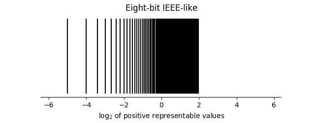
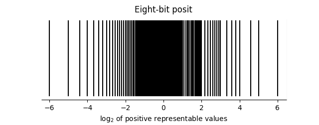
The graphs below give the distribution of 8-bit IEEE-like numbers and 8-bit posits on a log scale.

eight bit IEEE distribution

eight bit posit distribution

The distribution of IEEE-like numbers is asymmetric because much of the dynamic range comes from denormalized numbers.

The distributions of posits is approximately symmetrical. If a power of 2 is representable as a posit, so is its reciprocal. But you don’t have perfect symmetry because, for example, 3/2 is representable while 2/3 is not.

Other eight-bit formats

I had originally considered a 2-bit significand because Microsoft’s ms-fp8 format has a two-bit significand. After this post was first published it was suggested in the comments that an ieee<8, 4> float might be better than ieee<8, 2>, so let’s look at that. Let’s look at ieee<8, 3> too while we’re at it. And a posit<8, 1> too.

An ieee<8, 3> floating point number would have a maximum value of 7 and a minimum value of 2−6 = 1/64, a dynamic range of  2.7 decades. It would have 223 finite values, including two zeros, as well as 2 infinities as 30 NaNs.

An ieee<8, 4> floating point number would have a maximum value of 120 and a minimum value of 2−9 = 1/512, a dynamic range of 4.7 decades. It would have 239 finite values, including two zeros, as well as 2 infinities and 14 NaNs.

A posit<8, 1> would have a maximum value of 212 = 4096 and a minimum value of 1/4096, a dynamic range of  7.2 decades. Any 8-bit posit, regardless of the maximum number of exponent bits, will have 255 finite values and one infinity.

Near 1, an ieee<8, 4> has 3 significand bits, an ieee<8, 3> has 4, and a posit<8,1> has 4.

***

[1] Chung et al. Serving DNNs in Real Time at Datacenter Scale with Project Brainwave. Available here.