Scaling and Monte Carlo integration methods

Posted on 2 February 2018 by John

Here’s an apparent paradox. You’ll hear that Monte Carlo methods are independent of dimension, and that they scale poorly with dimension. How can both statements be true?

The most obvious way to compute multiple integrals is to use product methods, analogous to the way you learn to compute multiple integrals by hand. Unfortunately the amount of work necessary with this approach grows exponentially with the number of variables, and so the approach is impractical beyond modest dimensions.

The idea behind Monte Carlo integration, or integration by darts, is to estimate the area under a (high dimensional) surface by taking random points and counting how many fall below the surface. More details here. The error goes down like the reciprocal of the square root of the number of points. The error estimate has nothing to do with the dimension per se. In that sense Monte Carlo integration is indeed independent of dimension, and for that reason is often used for numerical integration in dimensions too high to use product methods.

Suppose you’re trying to estimate what portion of a (high dimensional) box some region takes up, and you know a priori that the proportion is in the ballpark of 1/2. You could refine this to a more accurate estimate with Monte Carlo, throwing darts at the box and seeing how many land in the region of interest.

But in practice, the regions we want to estimate are small relative to any box we’d put around them. For example, suppose you want to estimate the volume of a unit ball in n dimensions by throwing darts at the unit cube in n dimensions. When n = 10, only about 1 dart in 400 will land in the ball. When n = 100, only one dart out of 10⁷⁰ will land inside the ball. (See more here.) It’s very likely you’d never have a dart land inside the ball, no matter how much computing power you used.

If no darts land inside the region of interest, then you would estimate the volume of the region of interest to be zero. Is this a problem? Yes and no. The volume is very small, and the absolute error in estimating a small number to be zero is small. But the relative is 100%.

(For an analogous problem, see this discussion about the approximation sin(θ) = θ for small angles. It’s not just saying that one small number is approximately equal to another small number: all small numbers are approximately equal in absolute error! The small angle approximation has small relative error.)

If you want a small relative error in Monte Carlo integration, and you usually do, then you need to come up with a procedure that puts a larger proportion of integration points in the region of interest. One such technique is importance sampling, so called because it puts more samples in the important region. The closer the importance sampler fits the region of interest, the better the results will be. But you may not know enough a priori to create an efficient importance sampler.

So while the absolute accuracy of Monte Carlo integration does not depend on dimension, the problems you want to solve with Monte Carlo methods typically get harder with dimension.

Runge phenomena

Posted on 18 November 2017 by John

I’ve mentioned the Runge phenomenon in a couple posts before. Here I’m going to go into a little more detail.

First of all, the “Runge” here is Carl David Tolmé Runge, better known for the Runge-Kutta algorithm for numerically solving differential equations. His name rhymes with cowabunga, not with sponge.

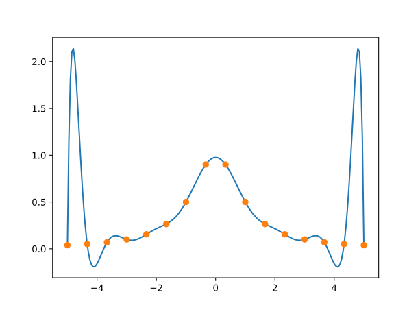
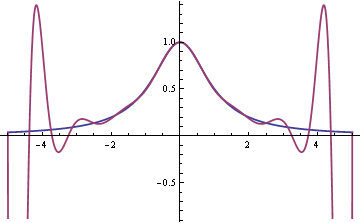
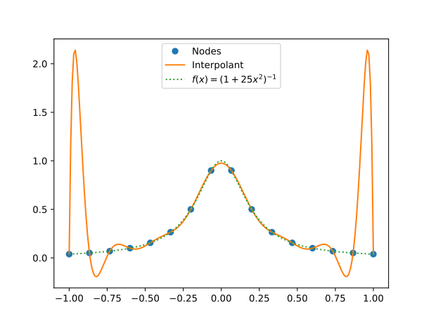
Runge showed that polynomial interpolation at evenly-spaced points can fail spectacularly to converge. His example is the function f(x) = 1/(1 + x²) on the interval [−5, 5], or equivalently, and more convenient here, the function f(x) = 1/(1 + 25x²) on the interval [−1, 1]. Here’s an example with 16 interpolation nodes.

Runge's example

Runge found that in order for interpolation at evenly spaced nodes in [−1, 1] to converge, the function being interpolated needs to be analytic inside a football-shaped [1] region of the complex plane with major axis [−1, 1] on the real axis and minor axis approximately [−0.5255, 0.5255] on the imaginary axis. For more details, see [2].

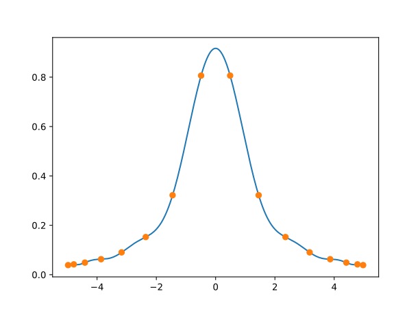
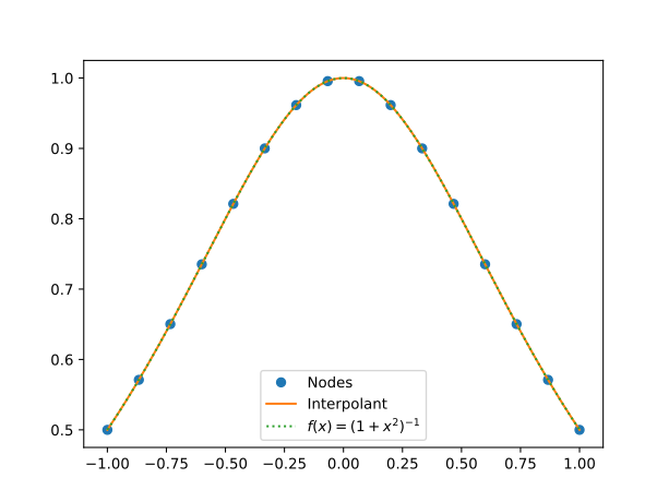
The function in Runge’s example has a singularity at 0.2i, which is inside the football. Linear interpolation at evenly spaced points would converge for the function f(x) = 1/(1 + x²) since the singularity at i is outside the football.

Runge's example

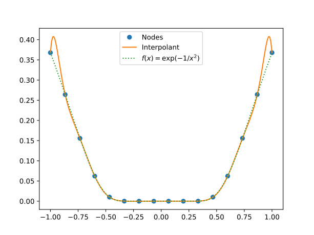
For another example, consider the function f(x) = exp(−1/x²) , defined to be 0 at 0. This function is infinitely differentiable but it is not analytic at the origin. With only 16 interpolation points as above, there’s a small indication of trouble at the ends.

Interpolating exp(-1/x^2)

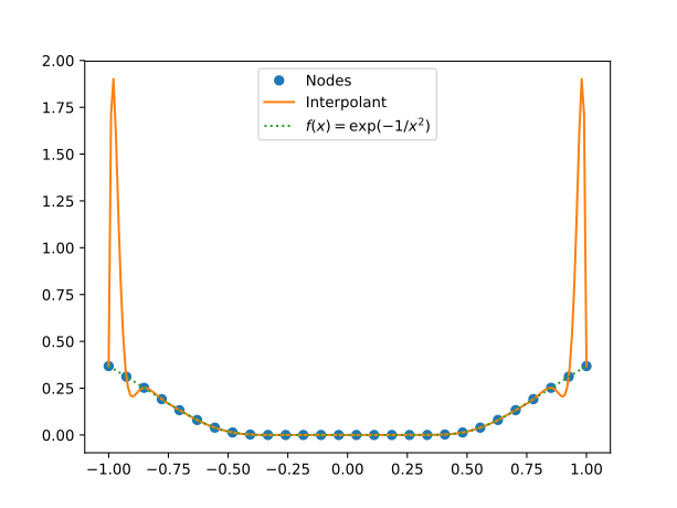
With 28 interpolation points in the plot below, the lack of convergence is clear.

Interpolating exp(-1/x^2)

The problem is not polynomial interpolation per se but polynomial interpolation at evenly-spaced nodes. Interpolation at Chebyshev points converges for the examples here. The location of singularities effects the rate of convergence but not whether the interpolants converge.

Related: Help with interpolation

***

[1] American football, that is. The region is like an ellipse but pointy at −1 and 1.

[2] Approximation Theory and Approximation Practice by Lloyd N. Trefethen

Chebyshev interpolation

Posted on 6 November 2017 by John

Fitting a polynomial to a function at more points might not produce a better approximation. This is Faber’s theorem, something I wrote about the other day.

If the function you’re interpolating is smooth, then interpolating at more points may or may not improve the fit of the interpolation, depending on where you put the points. The famous example of Runge shows that interpolating

f(x) = 1 / (1 + x²)

at more points can make the fit worse. When interpolating at 16 evenly spaced points, the behavior is wild at the ends of the interval.

Runge example

Here’s the Python code that produced the plot.

    import matplotlib.pyplot as plt
    from scipy import interpolate, linspace

    def cauchy(x):
        return (1 + x**2)**-1

    n = 16
    x = linspace(-5, 5, n) # points to interpolate at

    y = cauchy(x)
    f = interpolate.BarycentricInterpolator(x, y)

    xnew = linspace(-5, 5, 200) # points to plot at
    ynew = f(xnew)
    plt.plot(x, y, 'o', xnew, ynew, '-')
    plt.show()

However, for smooth functions interpolating at more points does improve the fit if you interpolate at the roots of Chebyshev polynomials. As you interpolate at the roots of higher and higher degree Chebyshev polynomials, the interpolants converge to the function being interpolated. The plot below shows how interpolating at the roots of T₁₆, the 16th Chebyshev polynomial, eliminates the bad behavior at the ends.

Runge example at Chebyshev nodes

To make this plot, we replaced x above with the roots of T₁₆, rescaled from the interval [-1, 1] to the interval [-5, 5] to match the example above.

    x = [cos(pi*(2*k-1)/(2*n)) for k in range(1, n+1)]
    x = 5*array(x)

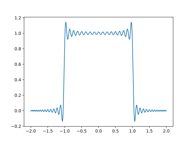
What if the function we’re interpolating isn’t smooth? If the function has a step discontinuity, we can see Gibbs phenomena, similar to what we saw in the previous post. Here’s the result of interpolating the indicator function of the interval [−1, 1] at 100 Chebyshev points. We get the same “bat ears” as before.

Gibbs phenomena for Chebyshev interpolation

Related: Help with interpolation

Yogi Berra meets Pafnuty Chebyshev

Posted on 31 October 2017 by John

I just got an evaluation copy of The Best Writing on Mathematics 2017. My favorite chapter was Inverse Yogiisms by Lloyd N. Trefethen.

Trefethen gives several famous Yogi Berra quotes and concludes that

Yogiisms are statements that, if taken literally, are meaningless or contradictory or nonsensical or tautological—yet nevertheless convey something true.

An inverse yogiism is the opposite,

[a] statement that is literally true, yet conveys something false.

What a great way to frame a chapter! Now that I’ve heard the phrase, I’m trying to think of inverse yogiisms. Nothing particular has come to mind yet, but I feel like there must be lots of things that fit that description. Trefethen comes up with three inverse yogiisms, and my favorite is the middle one: Faber’s theorem on polynomial interpolation.

Faber’s theorem is a non-convergence result for interpolants of continuous functions. Trefethen quotes several numerical analysis textbooks that comment on Faber’s theorem in a way that implies an overly pessimistic interpretation. Faber’s theorem is true for continuous functions in general, but if the function f being interpolated is smooth, or even just Lipschitz continuous, the theorem doesn’t hold. In particular, Chebyshev interpolation produces a sequence of polynomials converging to f.

A few years ago I wrote a blog post that shows a famous example due to Carle Runge that if you interpolate f(x) = 1/(1 + x²) over [−5, 5] with evenly spaced nodes, the sequence of interpolating polynomials diverges. In other words, adding more interpolation points makes the fit worse.

Here’s the result of fitting a 16th degree polynomial to f at evenly spaced nodes.

graph of f(x) and p16(x)

The error near the ends is terrible, though the fit does improve in the middle. If instead of using evenly spaced nodes you use the roots of Chebyshev polynomials, the interpolating polynomials do in fact converge, and converge quickly. If the kth derivative of f has bounded variation, then the error in interpolating f at n points is O(n^−k).

ODE solver as a functional fold

Posted on 2 June 2016 by John

One of the most widely used numerical algorithms for solving differential equation is the 4th order Runge-Kutta method. This post shows how the Runge-Kutta method can be written naturally as a fold over the set of points where the solution is needed. These points do not need to be evenly spaced.

Given a differential equation of the form

y' = f(t, y)

with initial condition y(t₀) = y₀, the 4th order Runge-Kutta method advances the solution by an amount of time h by

$y_{n+1} = y_n + \frac{h}{6}\left( k_{n1} + 2k_{n2} + 2k_{n3} + k_{n4}\right)$

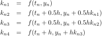
where

$k_{n1} &=& f(t_n, y_n) \\ k_{n2} &=& f(t_n + 0.5h, y_n + 0.5hk_{n1}) \\ k_{n3} &=& f(t_n + 0.5h, y_n + 0.5hk_{n2}) \\ k_{n4} &=& f(t_n + h, y_n + hk_{n3}) \\$

The Haskell code for implementing the accumulator function for foldl looks very much like the mathematical description above. This is a nice feature of the where syntax.

    rk (t, y) t' = (t', y + h*(k1 + 2.0*k2 + 2.0*k3 + k4)/6.0)
        where
            h  = t' - t
            k1 = f t y
            k2 = f (t + 0.5*h) (y + 0.5*h*k1)
            k3 = f (t + 0.5*h) (y + 0.5*h*k2)
            k4 = f (t + 1.0*h) (y + 1.0*h*k3)

Suppose we want to solve the differential equation y ‘ = (t² – y²) sin(y) with initial condition y(0) = -1, and we want to approximate the solution at [0.01, 0.03, 0.04, 0.06]. We would implement the right side of the equation as

     f t y = (t**2 - y**2)*sin(y)

and fold the function rk over our time steps with

    foldl rk (0, -1) [0.01, 0.03, 0.04, 0.06]

This returns (0.06, -0.9527). The first part, 0.06, is no surprise since obviously we asked for the solution up to 0.06. The second part, -0.9527, is the part we’re more interested in.

If you want to see the solution at all the specified points and not just the last one, replace foldl with scanl.

    scanl rk (0, -1) [0.01, 0.03, 0.04, 0.06]

This returns

    [(0.0, -1.0), (0.01, -0.9917), (0.03, -0.9756), (0.042, -0.9678), (0.06, -0.9527)]

As pointed out in the previous post, writing algorithms as folds separates the core of the algorithm from data access. This would allow us, for example, to change rk independently, such as using a different order Runge-Kutta method. (Which hardly anyone does. Fourth order is a kind of sweet spot.) Or we could swap out Runge-Kutta for a different ODE solver entirely just by passing a different function into the fold.

Next see how you could use a fold to compute mean, variance, skewness, and kurtosis in one pass through a stream of data using a fold.

MCMC burn-in

Posted on 25 January 2016 by John

In Markov Chain Monte Carlo (MCMC), it’s common to throw out the first few states of a Markov chain, maybe the first 100 or the first 1000. People say they do this so the chain has had a chance to “burn in.” But this explanation by itself doesn’t make sense. It may be good to throw away a few samples, but it could betray a lack of understanding to say a chain has “burned in.”

A Markov chain has no memory. That’s its defining characteristic: its future behavior depends solely on where it is, not how it got there. So if you “burn in” a thousand samples, your future calculations are absolutely no different than if you had started where there first thousand samples left off. Also, any point you start at is a point you might return to, or at least return arbitrarily close to again.

So why burn in? To enter a high probability region, a place where the states of the Markov chain are more representative of the distribution you’re sampling. When someone says a chain has “burned in,” that’s fine if they mean “has entered a high probability region.” And why do you want to enter such a region? Because you’re going to average some function of your samples:

$E[ f(X) ] \approx \frac{1}{n} \sum_{i=1}^n f(x_i)$

The result will be correct as n → ∞, but you’re going to stop after some finite n. When n is small, and your samples are in a low probability region, the average on the right might be a poor approximation to the expectation on the left.

The idea of burn-in is that you can start your MCMC procedure at some point chosen for convenience, one which might be out in the weeds, but then after a few iterations you’ll be in a high probability region. However, you don’t know that this will happen. It probably will happen, eventually, by definition: a random process spends most of its time where it spends most of its time! It is possible, though unlikely, that you could be in a lower probability region at the end of your burn-in period than at the beginning. Or maybe your chain is slowly moving toward a higher probability region, but you’re still not close at the end of your burn-in.

If you know where a high probability region is, just start there. Then you’ve “burned in” immediately. However, with a very complicated problem you might not know where a high probability region is. So you hope that a few steps of your chain will land you in a high probability region. And maybe it will. But if you understand your problem so poorly that you have no idea where the probability is concentrated, you’re going to have a hard time evaluating your results.

High-dimensional integration

Posted on 19 July 2015 by John

Numerically integrating functions of many variables almost always requires Monte Carlo integration or some variation. Numerical analysis textbooks often emphasize one-dimensional integration and, almost as a footnote, say that you can use a product scheme to bootstrap one-dimensional methods to higher dimensions. True, but impractical.

Traditional numerical integration routines work well in low dimensions. (“Low” depends on context, but let’s say less than 10 dimensions.) When you have the choice of a well-understood, deterministic method, and it works well, by all means use it. I’ve seen people who are so used to problems requiring Monte Carlo methods that they use these methods on low-dimensional problems where they’re not the most efficient (or robust) alternative.

Monte Carlo

Except for very special integrands, high dimensional integration requires either Monte Carlo integration or some variation such as quasi-Monte Carlo methods.

As I wrote about here, naive Monte Carlo integration isn’t practical for high dimensions. It’s unlikely that any of your integration points will fall in the region of interest without some sort of importance sampler. Constructing a good importance sampler requires some understanding of your particular problem. (Sorry. No one-size-fits-all black-box methods are available.)

Quasi-Monte Carlo (QMC)

Quasi-Monte Carlo methods (QMC) are interesting because they rely on something like a random sequence, but “more random” in a sense, i.e. more effective at exploring a high-dimensional space. These methods work well when an integrand has low effective dimension. The effective dimension is low when nearly all the action takes place on a lower dimensional manifold. For example, a function may ostensibly depend on 10,000 variables, while for practical purposes 12 of these are by far the most important. There are some papers by Art Owen that say, roughly, that Quasi-Monte Carlo methods work well if and only if the effective dimension is much smaller than the nominal dimension. (QMC methods are especially popular in financial applications.)

While QMC methods can be more efficient than Monte Carlo methods, it’s hard to get bounds on the integration error with these methods. Hybrid approaches, such as randomized QMC can perform remarkably well and give theoretical error bounds.

Markov Chain Monte Carlo (MCMC)

Markov Chain Monte Carlo (MCMC) is a common variation on Monte Carlo integration that uses dependent random samples. In many applications, such as Bayesian statistics, you’d like to be able to create independent random samples from some probability distribution, but this is not practical. MCMC is a compromise. It produces a Markov chain of dependent samples, and asymptotically these samples have the desired distribution. The dependent nature of the samples makes it difficult to estimate error and to determine how well the integration estimates using the Markov chain have converged.

(Some people speak of the Markov chain itself converging. It doesn’t. The estimates using the Markov chain may converge. Speaking about the chain converging may just be using informal language, or it may betray a lack of understanding.)

There is little theory regarding the convergence of estimates from MCMC, aside from toy problems. An estimate can appear to have converged, while an important region of the integration problem remains unexplored. Despite its drawbacks, MCMC is the only game in town for many applications.

***

Numerical integration consulting

Integration by Darts

Posted on 1 April 2015 by John

dartboard

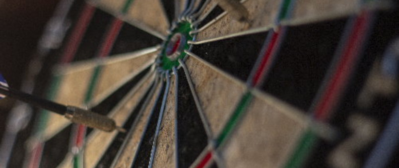
Monte Carlo integration has been called “Integration by Darts,” a clever pun on “integration by parts.” I ran across the phrase looking at some slides by Brian Hayes, but apparently it’s been around a while. The explanation that Monte Carlo is “integration by darts” is fine as a 0th order explanation, but it can be misleading.

Introductory courses explain Monte Carlo integration as follows.

Plot the function you want to integrate.
Draw a box that contains the graph.
Throw darts (random points) at the box.
Count the proportion of darts that land between the graph and the horizontal axis.
Estimate the area under the graph by multiplying the area of the box by the proportion above.

In principle this is correct, but this is far from how Monte Carlo integration is usually done in practice.

For one thing, Monte Carlo integration is seldom used to integrate functions of one variable. Instead, it is mostly used on functions of many variables, maybe hundreds or thousands of variables. This is because more efficient methods exist for low-dimensional integrals, but very high dimensional integrals can usually only be computed using Monte Carlo or some variation like quasi-Monte Carlo.

If you draw a box around your integrand, especially in high dimensions, it may be that nearly all your darts fall outside the region you’re interested in. For example, suppose you throw a billion darts and none land inside the volume determined by your integration problem. Then the point estimate for your integral is 0. Assuming the true value of the integral is positive, the relative error in your estimate is 100%. You’ll need a lot more than a billion darts to get an accurate estimate. But is this example realistic? Absolutely. Nearly all the volume of a high-dimensional cube is in the “corners” and so putting a box around your integrand is naive. (I’ll elaborate on this below. [1])

So how do you implement Monte Carlo integration in practice? The next step up in sophistication is to use “importance sampling.” [2] Conceptually you’re still throwing darts at a box, but not with a uniform distribution. You find a probability distribution that approximately matches your integrand, and throw darts according to that distribution. The better the fit, the more efficient the importance sampler. You could think of naive importance sampling as using a uniform distribution as the importance sampler. It’s usually not hard to find an importance sampler much better than that. The importance sampler is so named because it concentrates more samples in the important regions.

Importance sampling isn’t the last word in Monte Carlo integration, but it’s a huge improvement over naive Monte Carlo.

***

[1] So what does it mean to say most of the volume of a high-dimensional cube is in the corners? Suppose you have an n-dimensional cube that runs from −1 to 1 in each dimension and you have a ball of radius 1 inside the cube. To make the example a little simpler, assume n is even, n = 2k. Then the volume of the cube is 4^k and the volume of the sphere is π^k / k!. If k = 1 (n = 2) then the sphere (circle in this case) takes up π/4 of the volume (area), about 79%. But when k = 100 (n = 200), the ball takes up 3.46×10⁻¹⁶⁹ of the volume of the cube. You could never generate enough random samples from the cube to ever hope to land a single point inside the ball.

[2] In a nutshell, importance sampling replaces the problem of integrating f(x) with that of integrating (f(x) / g(x)) g(x) where g(x) is the importance sampler, a probability density. Then the integral of (f(x) / g(x)) g(x) is the expected value of (f(X) / g(X)) where X is a random variable with density given by the importance sampler. It’s often a good idea to use an importance sampler with slightly heavier tails than the original integrand.

Iterative linear solvers as metaphor

Posted on 25 June 2014 by John

Gaussian elimination is systematic way to solve systems of linear equations in a finite number of steps. Iterative methods for solving linear systems require an infinite number of steps in theory, but may find solutions faster in practice.

Gaussian elimination tells you nothing about the final solution until it’s almost done. The first phase, factorization, takes O(n^3) steps, where n is the number of unknowns. This is followed by the back-substitution phase which takes O(n^2) steps. The factorization phase tells you nothing about the solution. The back-substitution phase starts filling in the components of the solution one at a time. In application n is often so large that the time required for back-substitution is negligible compared to factorization.

Iterative methods start by taking a guess at the final solution. In some contexts, this guess may be fairly good. For example, when solving differential equations, the solution from one time step gives a good initial guess at the solution for the next time step. Similarly, in sequential Bayesian analysis the posterior distribution mode doesn’t move much as each observation arrives. Iterative methods can take advantage of a good starting guess while methods like Gaussian elimination cannot.

Iterative methods take an initial guess and refine it to a better approximation to the solution. This sequence of approximations converges to the exact solution. In theory, Gaussian elimination produces an exact answer in a finite number of steps, but iterative methods never produce an exact solution after any finite number of steps. But in actual computation with finite precision arithmetic, no method, iterative or not, ever produces an exact answer. The question is not which method is exact but which method produces an acceptably accurate answer first. Often the iterative method wins.

Successful projects often work like iterative numerical methods. They start with an approximation solution and iteratively refine it. All along the way they provide a useful approximation to the final product. Even if, in theory, there is a more direct approach to a final product, the iterative approach may work better in practice.

Algorithms iterate toward a solution because that approach may reach a sufficiently accurate result sooner. That may apply to people, but more important for people is the psychological benefit of having something to show for yourself along the way. Also, iterative methods, whether for linear systems or human projects, are robust to changes in requirements because they are able to take advantage of progress made toward a slightly different goal.

Root-finding with noisy functions

Posted on 14 June 2012 by John

Suppose you have function g(x) and you want to find x so that g(x) = 0. However, you don’t have direct access to g(x). Instead you can evaluate f(x) which is g(x) plus random noise. Typically f(x) would be an approximation of g(x) based on Monte Carlo simulation. I have spent countless hours solving problems like this.

One difficulty is that the value of f(x) will change every time you compute it. You might hunt down x and be sure you have it braketed between two values, only to find out you were wrong when you compute f(x) more accurately, say with more Monte Carlo steps.

Assume g(x), i.e. f(x) without noise, is monotone increasing. Assume also that f(x) is expensive to compute. Say each evaluation takes 20 minutes. The amplitude of the noise may vary with x.

Here’s a simple approach to trying to find where f(x) is zero. Use a bisection method, but stop when it looks like you’ve come as close as you can due to noise. If the monotonicity assumption is violated, use that as a signal that you’re within the resolution of the noise.

    # Assume a < b, fa = f(a) < 0, fb = f(b) > 0.
    def noisy_bisect(f, a, b, fa, fb, tolerance):
        if b-a < tolerance:
            return (a, b)
        mid = 0.5*(a+b)
        fmid = f(mid)
        if fmid < fa or fmid > fb:
            # Monotonicity violated. 
            # Reached resolution of noise.
            return (a, b)
        if fmid < 0:
            a, fa = mid, fmid
        else:
            b, fb = mid, fmid
        return noisy_bisect(f, a, b, fa, fb, tolerance)

The values of f(a) and f(b) are saved to avoid recalculation since they’re expensive to obtain.

You could experiment with this function as follows.

    from scipy.stats import norm
    from time import sleep

    # Gaussian distribution w/ mean 0 and standard deviation 0.01
    noise = norm(0, 0.01)

    def f(x):
        sleep(10) # wait 10 seconds
        return x**2 - 1 + noise.rvs()

    a = 0
    b = 3
    fa = f(a)
    fb = f(b)
    print noisy_bisect(f, a, b, fa, fb, 0.0001)

Without noise, the code would iterate until the zero is bracketed in an interval of width 0.0001. However, since the noise in on the order of 0.01, the method will typically stop when the bracket is a on the order of 0.01 wide, maybe a little smaller.

We could make the root-finding software a little faster by using a secant method rather than a bisection method. Instead of taking the midpoint, the secant method draws a line between (a, f(a)) and (b, f(b)) and uses the point where the line crosses the x-axis as the next guess.

A more sophisticated approach would be to increase the accuracy of f(x) over time. If f(x) is evaluated using N steps of a Monte Carlo simulation, the standard deviation of the noise is roughly proportional to 1/√N. So, for example, cutting the noise in half requires multiplying N by 4. You could get a rough bracket on the zero using a small value of N, then increase N as the bracket gets smaller. You could play with this by using a function like the following.

    def f(x, N):
        sleep(N) # wait N seconds
        noise = norm(0, 0.1/sqrt(N))
        return x**2 - 1 + noise.rvs()

You can make the noise as small as you’d like, but at a price. And the price goes up faster than the noise goes down, so it pays to not reduce the noise more than necessary.

Monte Carlo

Quasi-Monte Carlo (QMC)

Markov Chain Monte Carlo (MCMC)

More linear algebra posts