Randomized response and local differential privacy

Differential privacy protects user privacy by adding randomness as necessary to the results of queries to a database containing private data. Local differential privacy protects user privacy by adding randomness before the data is inserted to the database.

Using the visualization from this post, differential privacy takes the left and bottom (blue) path through the diagram below, whereas local differential privacy takes the top and right (green) path.

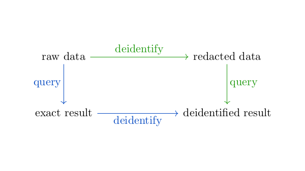
The diagram does not commute. Results are more accurate along the blue path. But this requires a trusted party to hold the identifiable data. Local differential privacy does not require trusting the recipient of the data to keep the data private and so the data must be deidentified before being uploaded. If you have enough data, e.g. telemetry data on millions of customers, then you can statistically afford to randomize your data before storing it.

I gave a simple description of randomized response here years ago. Randomized response gives users plausible deniability because their communicated responses are not deterministically related to their actual responses. That post looked at a randomized response to a simple yes/no question. More generally, you could have a a question with k possible answers and randomize each answer to one of ℓ different possibilities. It is not necessary that k = ℓ.

A probability distribution is said to be ε-locally differentially private if for all possible pairs of inputs x and x′ and any output y, the ratio of the conditional probabilities of y given x and y given x′ is bounded by exp(ε). So when ε is small, the probability of any given output conditional on each possible input is roughly the same. Importantly, the conditional probabilities are not exactly the same, and so one can recover some information about the unrandomized response in aggregate via statistical means. However, it is not possible to infer any individual’s unrandomized response, assuming ε is small.

In the earlier post on randomized response, the randomization mechanism and the inference from the randomized responses were simple. With multiple possible responses, things are more complicated. You could choose different randomization mechanisms and different inference approaches for different contexts and priorities.

With local differential privacy, users can share their data without trusting the data recipient to keep the data private; in a real sense the recipient isn’t receiving personal data at all. The recipient is receiving the output of a stochastic process which is weakly correlated with individual data, but isn’t receiving individual data per se.

Local differential privacy scales up well, but it doesn’t scale down well. When ε is small, each data contributor has strong privacy protection, but the aggregate data isn’t very useful unless so many individuals are represented in the data that the randomness added to the responses can largely be statistically removed.

Related posts

Earth mover’s distance

There are many ways to describe the distance between two probability distributions. The previous two posts looked at using the p-norm to measure the difference between the PDFs and using Kullbach-Leibler divergence. Earth mover’s distance (EMD) is yet another approach.

Imagine a probability distribution on ℝ² as a pile of dirt. Earth mover’s distance measures how different two distributions are by how much work it would take to reshape the pile of dirt representing one distribution into a pile of dirt representing the other distribution. Unlike KL divergence, earth mover’s distance is symmetric, and so it really is a distance. (EMD is a colorful name for what is more formally known as the Wasserstein metric.)

The concept of t-closeness in data privacy is based on EMD. Deidentification procedures such as k-anonymity that protect individual privacy may not protect group privacy. t-closeness measures the distribution of values of some attribute in a group and compares this distribution to that of the overall distribution using EMD.

Earth mover’s distance is difficult to compute, or even to rigorously define, when working in several dimensions, but in one dimension it is particularly simple. The 1-Wasserman distance between two probability distributions is simply the 1-norm distance between the corresponding CDFs.

W_1(X, Y) = \int_{-\infty}^\infty |F_X(x) - F_Y(x)|\, dx
There are p-Wasserstein metrics just as there are p-norms, but the case p = 1 is particularly simple and so we will focus on it for this post.

We can illustrate the univariate Wasserstein metric by returning to a problem in a recent post, namely now to optimally approximate a standard normal by a logistic distribution.

Logistic distribution example

One of the nice things about the logistic distribution is that its CDF is an elementary function. If X is a logistic distribution with mean 0 and scale s then the CDF is

F_X(x) = \frac{1}{1 + \exp(-x/s)}

The CDF of a normal distribution has no elementary form but can be written in terms of the complementary error function. If Z is a standard normal random variable, then

F_Z(x) = \mbox{erfc}( -x/\sqrt{2}) / 2

We get a distance of 0.05926 if we use the value of s  = 0.5513 obtained from moment matching here. The optimal value is s = 0.5867, a little smaller than the optimal values of s when minimizing the 1, 2, and ∞ norms which were around 0.61.

Related posts

KL divergence from normal to normal

The previous post looked at the best approximation to a normal density by normal density with a different mean. Dan Piponi suggested in the comments that it would be good to look at the Kullback-Leibler (KL) divergence.

The previous post looked at the difference from between two densities from an analytic perspective, solving the problem that an analyst would find natural. This post takes an information theoretic perspective. Just is p-norms are natural in analysis, KL divergence is natural in information theory.

The Kullback-Leibler divergence between two random variables X and Y is defined as

KL(X || Y) = -\int f_X(x) \log \frac{f_Y(x)}{f_X(x)} \, dx

There are many ways to interpret KL(X || Y), such as the average surprise in seeing Y when you expected X.

Unlike the p-norm distance, the KL divergence between two normal random variables can be computed in closed form.

Let X be a normal random variable with mean μX and variance σ²X and Y a normal random variable with mean μY and variance σ²Y. Then

KL(X || Y) = \log\frac{\sigma_Y}{\sigma_X} + \frac{\sigma_X^2 + (\mu_X - \mu_Y)^2}{2\sigma_Y^2} - \frac{1}{2}

If μX = 0 and σX = 1, then for fixed μY the value of σ²Y that minimizes KL(X || Y) is

\sigma_Y^2 = 1 + \mu_Y^2

KL divergence is not symmetric, hence we say divergence rather than distance. More on that here. If we want to solve the opposite problem, minimizing KL(X || Y), the optimal value of σ²Y is simply 1.

Normal approximation to normal

In my previous post on approximating a logistic distribution with a normal distribution I accidentally said something about approximating a normal with a normal.

Obviously the best approximation to a probability distribution is itself. As Norbert Wiener said “The best material model of a cat is another, or preferably the same, cat.”

But this made me think of the following problem. Let f be the density function of a standard normal random variable, i.e. one with mean zero and standard deviation 1. Let g be the density function of a normal random variable with mean μ > 0 and standard deviation σ.

For what value of σ does g best approximate f? Is it simply σ = 1? Does it depend on μ?

I looked at the 1, 2, and ∞ norms, and in each case the optimal value of σ is not 1, and the optimal value does depend on μ. When μ is close to 0, σ is close to 1, as you’d probably expect. But for larger μ the results are surprising.

For the 1-norm and 2-norm, the optimal value of σ increases with μ and reaches a maximum of 2, then remains constant.

For the ∞ norm, the optimal value of σ increases briefly then decreases.

Logistic / Normal approximation

In a recent post I pointed out that a soliton, a solution to the KdV equation, looks a lot like a normal density for fixed x. As someone pointed out in the comments, one way to look at this is that the soliton is exactly proportional to the density of a logistic distribution, and it’s well known that the logistic distribution is approximately normal.

Why?

Why might this approximation be useful?

You might want to approximate a normal distribution by a logistic distribution because the cumulative density function of the latter is an elementary function whereas the CDF of the former is not.

You might want to approximate a logistic distribution by a normal distribution because the normal distribution has nice, well-understood theoretical properties.

How?

If you wanted to approximate a logistic distribution by a normal, or vice versa, how would you do so? How large is the error in the approximation?

This post will answer these questions for four matching methods:

  1. Moment matching
  2. 1-norm
  3. 2-norm
  4. Sup-norm

We will find the value of the logistic scale parameter s that minimizes the distance between the logistic PDF

f(x, s) = sech²(x / 2s) / 4s

and that of the standard normal

g(x) = (2π)−1/2exp( − x²/2 )

by each of the criteria above. We set the scale parameter of the normal to 1 because the ratio of the optimal logistic scale to the normal scale is constant.

Moment matching

Let s be the scale parameter for the logistic distribution and let σ be the scale parameter for the normal distribution. We will assume both distributions have mean 0.

The variance of the logistic is π² s²/3 and the variance of the normal is σ². So moment matching requires

σ = π s / √3

or

s = √3 / π

since we’re setting σ = 1.

plot

How good is this approximation? That depends on how you measure the error, which we will explore below. We will see how it compares to the optimal solution under each criterion.

1-norm

It would be nice to calculate the 1-norm of the difference f(x, s) − g(x) then minimize this as a function of s. But that difference cannot be computed in closed form. At least Mathematica can’t compute it in closed form. So I found the minimum numerically.

plot

Moment matching sets s = 0.5513 and leads to a 1-norm error of 0.1087.

The optimal value of s for the 1-norm is s = 0.6137 which yields an error of 0.0665.

2-norm

plot
With moment matching s = 0.5513 and the 2-norm error is 0.05566.

The optimal value for the 2-norm is s = 0.61476 which yields a 2-norm error of 0.0006973.

sup-norm

The sup norm, a.k.a. min-max norm or ∞ norm, minimizes the maximum distance between the two functions.

plot

When s = 0.5513 the sup norm is 0.0545.

The optimal value of s for the sup norm is 0.6237 and yields a sup norm error of 0.01845.

Conclusion

We can improve on moment matching, for all three norms simultaneously, by using a larger value of s, such as 0.61.

If you have a normal(μ, σ) distribution and you want to approximate it by a logistic distribution, set the mean of the latter to μ and the scale to 0.61σ. If you care about a particular error measure, use the corresponding multiplier rather than 0.61.

If you want to approximate a logistic with mean μ and scale s by a normal, set the mean of the normal to μ and set σ = s/0.61.

Using classical statistics to avoid regulatory burden

On June 29 this year I said on Twitter that companies would start avoiding AI to avoid regulation.

Companies are advertising that their products contain AI. Soon companies may advertise that their projects are AI-free and thus exempt from AI regulations.

I followed that up with an article Three advantages of non-AI models. The third advantage I listed was

Statistical models are not subject to legislation hastily written in response to recent improvements in AI. The chances that such legislation will have unintended consequences are roughly 100%.

Fast forward four months and we now have a long, highly-detailed executive order, Executive Order 14110, effecting all things related to artificial intelligence. Here’s an excerpt:

… the Secretary [of Commerce] shall require compliance with these reporting requirements for: any model that was trained using a quantity of computing power greater than 1026 integer or floating-point operations, or using primarily biological sequence data and using a quantity of computing power greater than 1023 integer or floating-point operations; and any computing cluster that has a set of machines physically co-located in a single datacenter, transitively connected by data center networking of over 100 Gbit/s, and having a theoretical maximum computing capacity of 1020 integer or floating-point operations per second for training AI.

If a classical model can do what you need, you are not subject to any regulations that will flow out of the executive order above, not if these regulations use definitions similar to those in the executive order.

How many floating point operations does it take to train, say, a logistic regression model? It depends on the complexity of the model and the amount of data fed into the model, but it’s not 1020 flops.

Can you replace an AI model with something more classical like a logistic regression model or a Bayesian hierarchical model? Very often. I wouldn’t try to compete with Midjourney for image generation that way, but classical models can work very well on many problems. These models are much simpler—maybe a dozen parameters rather than a billion parameters—and so are much better understood (and so there is less fear of such models that leads to regulation).

I had a client that was using some complicated models to predict biological outcomes. I replaced their previous models with a classical logistic regression model and got better results. The company was so impressed with the improvement that they filed a patent on my model.

If you’d like to discuss whether I could help your company replace a complicated AI model with a simpler statistical model, let’s talk.

Differential entropy and privacy

Differential entropy is the continuous analog of Shannon entropy. Given a random variable X with density function fX, the differential entropy of X, denoted h(X), is defined as

h(X) = -\int f_X(x) \log_2 f_X(x)\, dx

where the integration is over the support of fX. You may see differential entropy defined using logarithm to a different base, which changes h(X) by a constant amount.

In [1] the authors defined the privacy of a random variable X, denoted Π(X), as 2 raised to the power h(X).

\Pi(X) = 2^{h(X)}

This post will only look at “privacy” as defined above. Obviously the authors chose the name because of its application to privacy in the colloquial sense, but here we will just look at the mathematics.

Location and scale

It follows directly from the definitions above that location parameters do not effect privacy, and scale parameters change privacy linearly. That is, for σ > 0,

\Pi(\sigma X + \mu) = \sigma \,\Pi(X)

If we divide by standard deviation before (or after) computing privacy then we have a dimensionless quantity. Otherwise there’s more privacy is measuring a quantity in centimeters than in measuring it in inches, which is odd since both contain the same information.

Examples

If X is uniformly distributed on an interval of length a, then h(X) = log2 a and Π(X) = a.

The privacy of a standard normal random variable Z is √(2πe) and so the privacy of a normal random variable with mean μ and variance σ² is σ√(2πe).

The privacy of a standard exponential random variable is 1, so the privacy of an exponential with rate λ is 1/λ.

Bounds

A well-known theorem says that for given variance, differential entropy is maximized by a normal random variable. This means that the privacy of a random variable with variance σ² is bounded above by σ√(2πe).

The privacy of a Cauchy random variable with scale σ is 4πσ, which is greater than σ√(2πe). This is does not contradict the statement above because the scaling parameter of a Cauchy random variable is not its standard deviation. A Cauchy random variable does not have and standard deviation.

Related posts

[1] Agrawal D., Aggrawal C. C. On the Design and Quantification of Privacy-Preserving Data Mining Algorithms, ACM PODS Conference, 2002. (Yes, the first author’s name contains one g and the second author’s name contains two.)

Best of N series

A couple days ago I wrote about the likelihood of the better team winning a best-of-five or best-of-seven series. That is, if the probability of X winning a game against Y is p > ½, how likely is it that X will win a majority of 5 games or a majority of 7 games.

This assumes the probability of winning each game is fixed and that each game is independent. Actual sports series are more complicated than that.

I was thinking about the baseball playoffs, and so I chose series of 5 and 7. But some tennis fans asked me to add series of 3. And others asked me to add series of more than 7.

As reported in the earlier post,the probability of X winning a series of N games is

\sum_{n > N-n} \binom{N}{n} p^n q^{N-n}

Here is a plot for series of 1, 3, 5, …, 29 games.

Best of N series

The blue diagonal line is the probability of winning each game, i.e. winning a 1-game series.

As you play longer series, the probability of the better team winning increases. Notice that you get the most lift from the diagonal line when playing a 3-game series, the orange line above. You get more lift going from 3 games to 5 games, from the orange line to the green line, though not as much. And as observed in the earlier post, you don’t get much improvement going from 5 games to 7 games, going from green to red.

Even with a series of 29 games, there’s a decent chance that the better team may not win the series, unless the better team is much better. The race is not always to the swift, nor the battle to the strong.

As you keep increasing the number of games N, the slope of the line in the middle becomes steeper, but slowly. You hit diminishing return immediately, with each additional pair of games making less and less difference. Still, the curve is getting steeper. Here’s the curve for a series of 499 games.

Best of 499 games

The slope of the curve in the middle is increasing in proportion to the square root of the number of games.

Related posts

Photo by J. Schiemann on Unsplash

Best-of-five versus Best-of-seven

Suppose that when Team X and Team Y play, the probability that X will win a single game is p and the probability that Y will win is q = 1 − p.

What is the probability that X will win the majority of a series of N games for some odd number N?

We know intuitively that the team more likely to win each game is more likely to win the series. But how much more likely?

We also know intuitively that the more games in the series, the more likely the better team will win. But how much more likely?

The probability of X winning a series of N games is

\sum_{n > N-n} \binom{N}{n} p^n q^{N-n}

It doesn’t matter that maybe not all games are played: some games may not be played precisely because it makes no difference whether they are played. For example, if one team wins the first three in a best-of-five series, the last two games are not played, but for our purposes we may imagine that they were played.

Let’s plot the probability of X winning a best-of-five series and a best-of-seven series.

The better team is more likely to win a series than a game. The probability of the better team winning a single game would be a diagonal line running from (0, 0) to (1, 1). The curves for a series are below this line to the left of 0.5 and above this line to the right of 0.5. But the difference between a best-of-five and a best-of-seven series is small.

Here’s another plot looking at the difference in probabilities, probability of winning best-of-seven minus probability of winning best-of-five.

The maximum difference is between 3% and 4%.

This assumes the probability of winning a game is constant and that games are independent. This is not exactly the case in, for example, the World Series in which human factors make things more complicated.

Related posts

U statistics and a new paper by Terence Tao

Terence Tao has a new paper out that relates to a couple things I’ve written about recently.

Elementary symmetric polynomials came up when developing the general equations for tangent sum and hyperbolic tangent sum. The latter post goes into more detail.

Before that, means of symmetric functions, not necessarily elementary polynomials or even polynomials, came up in the context of U-statistics.

Now combine these and you have means of elementary symmetric polynomials. This is what Tao just wrote about. Here is his blog post announcing his paper.

There are several inequalities satisfied by means of elementary symmetric named after Maclauren and Newton. If the inequalities don’t go all the way back to these two men, presumably they are a direct continuation of work they started.

The Maclauren and Newton inequalities require arguments to be non-negative; Tao allows arguments to possibly be negative.

U-statistics are not necessarily the means of elementary symmetric polynomials. But for those U-statistics that are, Tao’s new paper may imply new results. That is, Tao’s new paper has implications for statistics.