Correlation of two sine waves

What is the correlation of two sine waves that differ in phase? The result itself is interesting, and the calculation along the way shows tricks to avoid calculating integrals.

sines slightly out of phase

The correlation of two periodic signals, f and g, is

\frac{ \int \left( f - \mu_f\right) \left( g - \mu_g\right) \, dt } { \left( \int (f - \mu_f)^2\, dt \right)^{1/2} \left( \int (g - \mu_g)^2\, dt \right)^{1/2} }

where the integral is over a period of the two functions. For functions known at discrete points this would be a sum rather than an integral, but in this case we have continuous signals so we integrate.

In our case the two functions are f(t) = sin(t) and g(t) = sin(t + φ) and the integrals are over [0, 2π]. Both functions have average value 0, so the μ terms go away.

We use a trig identity to expand the numerator:

\sin\theta_1 \sin \theta_2 = \frac{1}{2} \left( \cos(\theta_1-\theta_2) - \cos(\theta_1 + \theta_2) \right)

In our case θ1 = t and θ2 = t + φ and so the numerator becomes

\frac{1}{2} \int_0^{2\pi} \cos\phi - \cos(2t + \phi) \, dt = \pi \cos \phi

The first part of the integral is integrating a constant (with respect to t) and so becomes the constant times the length of the integration range. The second part of the integral is zero because it is integrating a cosine over two periods.

Now for the denominator. Over a full period, sin2(t) and cos2(t) take on the same values, just shifted. So the integral of sin2(t) is half the integral of sin2(t) + cos2(t) = 1. Therefore

\int_0^{2\pi} \sin^2 t\, dt = \frac{1}{2}(2\pi) = \pi

and the same argument shows that the integral of sin2(t + φ) is also π. So our correlation is simply cos φ: the correlation of two out-of-phase sine waves is the cosine of their phase difference. It may be a little surprising that it works out to be so simple, but the result makes sense. When φ = 0, or any multiple of 2π, the waves are identical and so the correlation should be 1. When φ = π, or an odd multiple of π, the two waves are perfectly out of phase, and so the correlation should be −1. In between these extremes the correlation oscillates, in fact it is a cosine.

Energy in frequency modulated signals

In an earlier post we proved that if you modulate a cosine carrier by a sine signal you get a signal whose sideband amplitudes are given by Bessel functions. Specifically:

\cos( 2\pi f_c t + \beta \sin(2\pi f_m t) ) = \sum_{k=-\infty}^\infty J_n(\beta) \cos(2\pi(f_c + nf_m)t)

When β = 0, we have the unmodulated carrier, cos(2π fct), on both sides. When β is positive but small, J0(β) is near 1, and so the frequency component corresponding to the carrier is only slightly diminished. Also, the sideband amplitudes, the values of Jn(β) for n ≠ 0, are small and decay rapidly as |n| increases. As β increases, the amplitude of the carrier component decreases, the sideband amplitudes increase, and the sidebands decay more slowly.

We can be much more precise: the energy in the modulated signal is the same as the energy in the unmodulated signal. As β increases, more energy transfers to the sidebands, but the total energy stays the same. This conservation of energy result applies to more complex signals than just pure sine waves, but it’s easier to demonstrate in the case of a simple signal.

Proof

To prove the energy stays constant, we show that the sum of the squares of the coefficients of the cosine components is the same for the modulated and unmodulated signal.The unmodulated signal is just cos(2π fct), and so the only coefficient is 1. That means we have to prove

 \sum_{n=-\infty}^\infty J_n(\beta)^2 = 1

This is a well-known result. For example, it is equation 9.1.76 in Abramowitz and Stegun. We’ll show how to prove it from first principles. We’ll actually prove a more general result, the Newmann-Schläffi addition formula, then show our result follows easily from that.

Newmann-Schläffi addition formula

Whittaker and Watson define the Bessel functions by their generating function:

\exp\left(\frac{z}{2}\left(t - \frac{1}{t}\right)\right) = \sum_{n=-\infty}^\infty t^n J_n(z)

This means that when you expand the expression on the left as a power series in t, whatever is multiplied by tn is Jn(z) by definition. (There are other ways of defining the Bessel functions, but this way leads quickly to what we want to prove.)

We begin by factoring the Bessel generating function applied to zw.

\exp\left(\frac{z+w}{2}\left(t - \frac{1}{t}\right)\right) = \exp\left(\frac{z}{2}\left(t - \frac{1}{t}\right)\right) \exp\left(\frac{w}{2}\left(t - \frac{1}{t}\right)\right)

Next we expand both sides as power series.

\sum_{n=-\infty}^\infty t^n J_n(z+w) = \sum_{j=-\infty}^\infty t^j J_j(z) \sum_{k=-\infty}^\infty t^k J_k(w)

and look at the terms involving tn on both sides. On the left this is Jn(zw). On the right, we multiply two power series. We will get a term containing tn whenever we multiply terms tj and tk where j and k sum to n.

 J_n(z+w) = \sum_{j+k = n} J_j(z) J_k(w) = \sum_{m=-\infty}^\infty J_m(z) J_{n-m} J(w)

The equation above is the Newmann-Schläffi addition formula.

Sum of squared coefficients

To prove that the sum of the squared sideband coefficients is 1,  we apply the addition formula with n = 0, z = β, and w = -β.

1 = J_0(\beta - \beta) = \sum_{m=-\infty}^\infty J_m(\beta) J_{-m}(-\beta) = \sum_{m=-\infty}^\infty J_m(\beta)^2

This proves what we were after:

 \sum_{n=-\infty}^\infty J_n(\beta)^2 = 1

We used a couple facts in the last step that we haven’t discussed. The first was that J0(0) = 1. This follows from the generating function by setting z to 0 and taking the limit as t → 0. The second was that Jm(-β) = Jm(β). You can also see this from the generating function since negating z has the same effect as swapping t and 1/t.

More DSP posts

Quantifying Loudness

How do you quantify how loud a sound is? Sounds like a simple question, but it’s not.

What is loudness?

It’s not hard to measure the physical intensity of a sound, but loudness is the perceived intensity of a sound. It is not a physical phenomena but a psychological phenomena.

Loudness is subjective, but not entirely so. There is general consensus regarding what it means for two sounds to be equally loud, and even for ratios, such as saying when one sound is twice as loud as the other. Loudness is quantifiable, but not easily so.

What does loudness depend on?

Loudness depends on several properties of a sound, such as its frequency, bandwidth, and duration. Loudness must depend on frequency because sounds that are too low or too high have no loudness at all because we simply cannot hear them. But even with the range of audible frequencies, loudness varies quite a bit by pitch. The graph below, via Wikipedia, shows equal loudness contours. The blue lines are from work by Fletcher and Munson in 1937. The red lines are the revised curves per the ISO 226:2003 standard.

Fletcher-Munson curves

The horizontal axis is frequency in Hz and the vertical axis is sound pressure level in decibels. The contour lines represent combinations of frequency and sound pressure level that are perceived to be equally loud. If a tuba and a flute sound equally loud, the sound pressure level coming from the tuba is much higher.

Notice that the curves are not parallel, They’re much closer together for low frequencies than for midrange frequencies, though they are roughly parallel for high frequencies. This means that if you recorded a piano, for example, playing each of its keys at equal loudness, the pitches wouldn’t sound equally loud unless you played the recording back at its original volume.

Complexities and simplifications

As complicated as this is, it’s still a simplification. It is based on pure tones, simple sine waves. A single musical instrument, much less an orchestra or a jackhammer, are more complicated. Loudness is highly nonlinear, and so you cannot say that the loudness of two sounds is the sum of their individual loudnesses. A-weighting is a relatively simple way to convert sound pressure levels to loudness, but is only accurate for pure tones at fairly low loudness levels.

To simplify thing further, consider a single pure tone, a sine wave at 1 kHz. (This is almost two octaves above middle C. See details here.) Loudness level in phons is defined to match sound pressure level in decibels for a 1 kHz pure tone. So a sound has a loudness level of 40 phons, for example, if it is perceived to be as loud as a pure 1 hKz tone at 40 dB.

At 1 kHz, loudness increases by a factor of 2 for every 10 dB increase in sound pressure level. But because nothing is simple in psychoacoustics, even this is a simplification. It only holds for sounds with loudness level 40 dB or greater. A quiet room is around 40 phons, so the added complications below 40 phons may not be relevant in many applications.

A pure tone at 1 kHz and 20 dB sounds more than four times softer than the same tone at 40 dB. The definition of loudness level in phons still holds below 40 phons. An oboe has a loudness level of 20 phons if it has the same loudness as a sine wave with frequency 1 kHz and sound pressure level 20 dB. But an oboe at 30 phons will sound more than twice as loud as one at 20 phons.

Update: New blog post comparing guitar samples at the same sound pressure level but with differing loudness and sharpness.

Summary

So where are we as far as calculating loudness? We’ve said a lot about what you can’t do, what complications have to be considered. But we’ve concluded this much: for a pure 1 kHz tone, the loudness in phons equals (by definition) the sound pressure level in decibels. And we’ve said how in principle you could define the loudness of other sounds: compare them to a 1 kHz tone that’s just as loud. We haven’t said how to compute this, only how you could determine it empirically.

In future posts I may write about how you do this using the ISO 532B standard or the newer ANSI S3.4-2007 standard.

Related links

Analyzing an FM signal

radio dial

Frequency modulation combines a signal with a carrier wave by changing (modulating) the carrier wave’s frequency.

Starting with a cosine carrier wave with frequency fc Hz and adding a signal with amplitude β and frequency fm Hz results in the combination

\cos( 2\pi f_c t + \beta \sin(2\pi f_m t) )

The factor β is known as the modulation index.

We’d like to understand this signal in terms of cosines without any frequency modulation. It turns out the result is a set of cosines weighted by Bessel functions of β.

\cos( 2\pi f_c t + \beta \sin(2\pi f_m t) ) = \sum_{k=-\infty}^\infty J_n(\beta) \cos(2\pi(f_c + nf_m)t)

Component amplitudes

We will prove the equation above, but first we’ll discuss what it means for the amplitudes of the cosine components.

For small values of β, Bessel functions decay quickly, which means the first cosine component will be dominant. For larger values of β, the Bessel function values increase to a maximum then decay like one over the square root of the index. To see this we compare the coefficients for modulation index β = 0.5 and β = 5.0.

First, β = 0.5:

and now for β = 5.0:

For fixed β and large n we have

J_n(\beta) \approx \frac{\beta^n}{2^n \, n!}

and so the sideband amplitudes eventually decay very quickly.

Update: See this post for what the equation above says about energy moving from the carrier to sidebands.

Proof

To prove the equation above, we need three basic trig identities

\cos(A + B) &=& \cos A \cos B - \sin A \sin B \\ 2\cos A \cos B &=& \cos(A-B) + \cos(A+B) \\ 2\sin A \sin B &=& \cos(A-B) - \cos(A+B)

and three Bessel function identities

\cos( z \sin \theta) &=& J_0(z) + 2\sum_{k=1}^\infty J_{2k}(z) \cos(2k\theta) \\ \sin( z \sin \theta) &=& 2\sum_{k=0}^\infty J_{2k+1}(z) \sin((2k+1)\theta) \\ J_{-n}(z) &=& (-1)^n J_n(z)

The Bessel function identities above can be found in Abramowitz and Stegun as equations 9.1.42, 9.1.43, and 9.1.5.

And now the proof. We start with

\cos( 2\pi f_c t + \beta \sin(2\pi f_m t) )

and apply the sum identity for cosines to get

\cos(2\pi f_c t) \cos(\beta \sin(2\pi f_m t)) - \sin(2\pi f_c t) \sin(\beta \sin(2\pi f_m t))

Now let’s take the first term

 \cos(2\pi f_c t) \cos(\beta \sin(2\pi f_m t))

and apply one of our Bessel identities to expand it to

J_0(\beta) \cos(2\pi f_c t) + \sum_{k=1}^\infty J_{2k}(\beta) \left\{ \cos(2\pi (f_c - 2k f_m)t) + \cos(2\pi(f_c + 2k f_m)t) \right\}

which can be simplified to

\sum_{n \,\, \mathrm{even}} J_n(\beta) \cos(2\pi(f_c + nf_m)t)

where the sum runs over all even integers, positive and negative.

Now we do the same with the second half of the cosine sum. We expand

\sin(2\pi f_c t) \sin(\beta \sin(2\pi f_m t))

to

\sum_{k=1}^\infty J_{2k+1}(\beta) \left\{ \cos(2\pi (f_c - (2k+1) f_m)t) - \cos(2\pi(f_c + (2k+1) f_m)t) \right\}

which simplifies to

\sum_{k=1}^\infty J_{2k+1}(\beta) \left\{ \cos(2\pi (f_c - (2k+1) f_m)t) - \cos(2\pi(f_c + (2k+1) f_m)t) \right\}

where again the sum is over all (odd this time) integers. Combining the two halves gives our result

\cos( 2\pi f_c t + \beta \sin(2\pi f_m t) ) = \sum_{k=-\infty}^\infty J_n(\beta) \cos(2\pi(f_c + nf_m)t)

***

More on mathematics and radio.

Fourier transform of a function on a graph

What is a Fourier transform at its core? An expansion of function in terms of eigenfunctions of the Laplacian. For a function on the real line, the Laplacian is simply the second derivative. The functions mapped to multiples of themselves by taking second derivatives are sines and cosines of various frequencies. A Fourier series is a change of basis, using as basis vectors those functions who behave the simplest under the second derivative.

The Fourier transform of a function on a graph is also a change of basis, expanding a discrete function in terms of eigenvalues of the Laplacian, in this case the graph Laplacian.

The Fourier transform of a function f, evaluated at a frequency ω, is the inner product of f with the eigenfunction exp(2πiωt).

\hat{f}(\omega) = \langle f, \exp(2\pi i \omega t) \rangle = \int_{-\infty}^\infty f(t) \exp(-2\pi i \omega t) \, dx

The inner product of two complex functions f and g is the integral of the product of f and the conjugate of g. Conjugation is why exp(2πiωt) became exp(-2πiωt).

The Fourier transform of a discrete function f on a graph, evaluated at an eigenvalue λi, is the inner product of f (i.e. the vector of values of f at each node) with the eigenvector associated with λi.

\hat{f}(\lambda_i) = \langle f, v^*_i \rangle = \sum_{j=1}^N f(j) v_i^*(j)

Here the inner product is a discrete sum rather than an integral. As before, we take the complex conjugate of the second item in the product.

The eigenvectors associated with the smallest eigenvalues of the graph Laplacian are analogous to low frequency sines and cosines. The eigenvalue components corresponding to nearly vertices in a graph should be close together. This analogy explains why spectral coordinates work so well.

Related posts

Discrete Laplace transform

The relationship between the discrete Laplace transform and discrete Fourier transform is not quite the same as that between their continuous counterparts.

Continuous Fourier and Laplace transforms

The continuous versions of the Fourier and Laplace transforms are given as follows.

Fourier transform:

{\cal F}(f)(\omega) = \int_{-\infty}^\infty \exp(-i\omega x) f(x)\, dx

Laplace transform:
{\cal L}(f)(s) = \int_0^\infty \exp(-s x) f(x)\, dx

The Fourier transform is defined several ways, and I actually prefer the convention that puts a factor of 2π in the exponential, but the convention above makes the analogy with Laplace transform simpler. There are two differences between the Fourier and Laplace transforms. The Laplace transform integrates over only half the real line, compared to the entire real line for Fourier. But a variation on the Laplace transform, the Bilateral Laplace transform integrates over the entire real line. The Bilateral Laplace transform at s is simply the Fourier transform at xis. And of course the same is true for the (one-sided) Laplace transform if the function f is only non-zero for positive values.

I’ve encountered the Fourier transform more in application, and the Laplace transform more in teaching. This is not to say the Laplace transform isn’t used in practice; it certainly is used in applications. But the two transforms serve similar purposes, and the Laplace transform is easier to teach. Because the factor exp(-sx) decays rapidly, the integral defining the Laplace transform converges for functions where the integral defining the Fourier transform would not. Such functions may still have Fourier transforms, but the transforms require distribution theory whereas the Laplace transforms can be computed using basic calculus.

Discrete Fourier and Laplace Transforms

There’s more difference between the discrete versions of the Fourier and Laplace transforms than between the continuous versions.

The discrete Fourier transform (DFT) approximates the integral defining the (continuous) Fourier transform with a finite sum. It discretizes the integral and truncates its domain. The discrete Laplace transform is an infinite sum. It discretizes the integral defining the Laplace transform, but it does not truncate the domain. Given a step size η > 0, the discrete Laplace transform of f is

{\cal L}_\eta(f)(s) = \eta \sum_{n=0}^\infty \exp(-sn\eta) f(n\eta)

The discrete Laplace transform isn’t “as discrete” as the discrete Fourier transform. The latter takes a finite sequence and returns a finite sequence. The former evaluates a function at an infinite number of points and produces a continuous function.

The discrete Laplace transform is used in applications such as signal processing, as well as in the theory of analytic functions.

Connection with the z-transform and generating functions

If η = 1 and z = exp(-s), the discrete Laplace transform becomes the z-transform of the values of f at non-negative integers. And if we replace z with 1/z, or equivalently set z = exp(s) instead of z = exp(-s), we get the generating function of the values of f at non-negative integers.

z-transforms are common in digital signal processing, while generating functions are common in combinatorics. They are essentially the same thing.

Visualizing the DFT matrix

The discrete Fourier transform (DFT) of length N multiplies a vector by a matrix whose (j, k) entry is ωjk where ω = exp(−2πi/N), with j and k running from 0 to − 1. Each element of the matrix is a rotation, so if N = 12, we can represent each element by an hour on a clock. The angle between the hour hand and minute hand corresponds to the phase of the matrix entry. We could also view each element as a color around a color wheel. The image below does both.

The matrix representing the inverse of the DFT is the conjugate of the DFT matrix (divided by Nf, but we’re only looking at phase here, so we can ignore this rescaling.) The image below displays the DFT matrix on the left and it’s inverse on the right.

Taking the conjugate amounts to making all the clocks run backward.

The DFT is often called the FFT. Strictly speaking, the FFT is an algorithm for computing the DFT. Nobody computes a DFT by multiplying by the DFT matrix, because the FFT is faster. The DFT matrix has a lot of special structure, which the FFT takes advantage of to compute the product faster than using ordinary matrix multiplication.

By the way, there are Unicode characters for clock times on the hour, U+1F550 through U+1F55B. I created the image above by writing a script that put the right characters in a table. The colors have HSL values where H is proportional to the angle and S = L =0.8.

Relating Fourier series and Fourier transforms

Fourier series and Fourier transforms may seem more different than they are because of the way they’re typically taught. Fourier series are presented more as a representation of a function, not a transformation. Here’s a function on an interval. We can write it as a sum of sines and cosines, just as we can write a function as a sum of powers in a power series. There’s not much emphasis on the coefficients per se. They appear inside a sum, but don’t get much attention on their own.

Fourier transforms, on the other hand, are presented as genuine transforms. Here’s a function, and here’s its transform, another function. One’s a function of time, the other a function of frequency. Or maybe both are presented as representations of the same function in two different domains, the time domain and the frequency domain.

You could think of the Fourier series as a kind of transform, taking a periodic function and mapping it to an infinite sequence, the Fourier series coefficients. And you could think of the Fourier transform as being a kind of continuous set of coefficients for representing a function, if you interpret the inversion theorem the right way.

Here are a couple connections between Fourier series and Fourier transforms. Start with a function f on an interval and compute its Fourier series. The Fourier series is periodic, so we could think of f as periodic, even though we only care about f on the interval. Instead, let’s think of extending f to be 0 everywhere outside the interval. Now we take the Fourier transform of f. The Fourier series coefficients are the Fourier transform of f evaluated at integer arguments.

Now let’s go back to thinking of f as a periodic function. What would it’s Fourier transform look like? In classical analysis, you can’t do that. Periodic functions have Fourier series but they don’t have Fourier transforms because the integral defining the latter does not converge. But by the magic of tempered distributions, we can indeed take the Fourier transform of a periodic function. The result is a weighted sum of delta distributions at each integer, and the coefficient of the delta distribution at n is the nth Fourier series coefficient.

The proof of the claim in the previous paragraph is simple once you understand the sha function Ш. Start with a function f defined on a unit interval and extended to be zero outside that interval. Convolving f with Ш make a periodic function f*Ш extending f. The Fourier transform of a convolution is the product of the convolutions. The Fourier transform of f is simply its classical Fourier transform F. The Ш function is its own Fourier transform, so the transform of f*Ш is FШ. Multiplying a function by Ш samples that function, and the samples of F are the Fourier coefficients of the Fourier series of f*Ш, the periodic extension of f.

An example of coming full circle

Here’s an interesting line from Brad Osgood:

Isn’t it a little embarrassing that multibillion dollar industries seem to depend on integrals that don’t converge?

In context, he’s not saying that huge companies are blithely using bad math. Some are, but that’s not what he’s getting at here. His discussion is an example of coming full circle, where experts and novices come to the same conclusion for different reasons.

The divergent integrals Osgood refers to are Fourier transforms of certain functions. A beginner might not notice that said integrals don’t converge. An expert knows that the calculations are justified by a more sophisticated theory. Someone in-between would have objections. Experts can be casual, not because they’re ignorant of technical difficulties but because they’ve mastered these difficulties. [1]

The expert in Fourier analysis has all the technicalities in the back of his or her mind. Often these don’t need to be explicitly exercised. You can blithely go about using formal calculations that aren’t justified by the classical theory.

But the expert doesn’t entirely come full circle, not in the sense of walking in circles in the woods. It’s more like winding around a parking garage, coming back to the same (x, y) location but one level up. Sometimes the expert needs to pull out the technical machinery to avoid an error the beginner could fall into. The theory of tempered distributions, for example, doesn’t justify every calculation a novice might try.

***

[1] In a nutshell, here’s the theory that justifies apparently sloppy calculations with Fourier transforms. The key is to view the function you want to transform not as a function on the real line but as a tempered distribution, a linear functional on the space of smooth, rapidly decaying test functions. A function acts on a test function by forming their product and integrating. Then use Parseval’s theorem from the classical theory as the definition in this new context, moving the transform operation from the original function to the test function. Simple, right?

The Dirac comb or Sha function

shaThe sha function, also known as the Dirac comb, is denoted with the Cyrillic letter sha (Ш, U+0428). This letter was chosen because it looks like how people visualize the function, a long series of vertical spikes. The function is called the Dirac comb for the same reason. This function is very important in Fourier analysis because it relates Fourier series and Fourier transforms. It relates sampling and periodization.  It’s its own Fourier transform, and with a few qualifiers discussed later, the only such function.

The Ш function, really the Ш distribution, is defined as
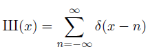
sha(x) = \sum_{n=-\infty}^\infty \delta(x-n)

Here δ(xn) is the Dirac delta distribution centered at n. The action of δ(xn) on a test function is to evaluate that function at n. You can envision Ш as an infinite sequence of spikes, one at each integer. The action of Ш on a test function is to add up its values at every integer.

Sampling

The product of Ш with a function f is a new distribution whose action on a test function φ is the sum of f φ over all integers. Or you could think of the distribution as a sort of clothesline on which to hang the sampled values of f, much the way a generating function works.

Periodizing

Next let’s look at a function f that lives on [0, 1], i.e. is zero everywhere outside the unit interval. The convolution of f with δ(xn) is f(xn), i.e. a copy of f shifted over to live on the interval [n, n+1]. So by taking the convolution with Ш, we create copies of f all over the real line. We’ve made f into a periodic function. So instead of saying “the function f extended to create a periodic function” you can simply say f*Ш.

Fourier transform

Now let’s think about the Fourier transform of Ш. The Fourier transform of δ(x) is 1, i.e. the function equal to 1 everywhere [1].  (The more concentrated a function is, the more spread out its Fourier transform. So if you have an infinitely concentrated function δ, its Fourier transform is perfectly flat, 1. You can calculate the transform rigorously, this is the intuition.) If you shift a function by n, you rotate its Fourier transform by exp(-2πinω). So we can compute the transform of Ш:

Fourier transform of sha = \sum_{n=-\infty}^\infty \exp(-2\pi i n \omega)

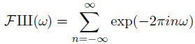
This equation only makes sense in terms of distributions. The right hand side does not converge in the classical sense; the individual terms don’t even go to zero, since each term has magnitude 1. So what kind of distribution is this thing on the right side? It is in fact the Ш function again, though this is not obvious.

To see that the exponential sum is actually the Ш function, i.e. that Ш is its own Fourier transform, we need to back up a little bit and define Fourier transform of a distribution. As usual with distributions, we take a classical theorem and turn it into a definition in a broader context.

For absolutely integrable functions, we have

\int_{-\infty}^ \infty \hat{f}(x) \, \varphi(x) \, dx = \int_{-\infty}^ \infty f(x) \, \hat{ \varphi }(x) \, dx

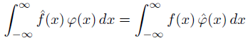
where the hat on top of a function indicates its Fourier transform. Inspired by the theorem above, we define the Fourier transform of a distribution f to be the functional whose action on a test function φ is given below.

 \hat{f} : \varphi \mapsto \int_{-\infty}^ \infty f(x) \, \hat{ \varphi }(x) \, dx

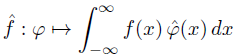
As we noted in a previous post, the integral above can be taken literally if f is a distribution associated with an ordinary function, but in general it means the application of the linear functional to the test function.

As a distribution, exp(-2πinω) acts on a test function φ by integrating against it. From the definition of a (classical) Fourier transform, this gives the Fourier transform of φ evaluated at n. So the Fourier transform of Ш acts on φ by summing the values of φ’s Fourier transform over all integers. By the Poisson summation formula, this is the same as summing the values of φ itself over all integers. Which is the same as applying Ш. So the Fourier transform of Ш has the same effect on test functions as Ш. In other words, Ш is its own Fourier transform.

Uniqueness

We haven’t been explicit about where our test functions come from. We require that xn φ(x) goes to zero as x goes to ±∞ for any positive integer n. These are called functions of rapid decay. And the distributions we define as linear functionals on such test functions are called tempered distributions.

The Ш distribution is essentially unique. Any tempered distribution with period 1 that equals its own Fourier transform must be a multiple of Ш.

***

[1] All Fourier transform calculations here use the convention I call (-1, τ, 1) in these notes on various definitions. This may be the most common definition, though there are several minor variations in common use.