Suppose you draw samples from two populations, one of which has a wider probability distribution than the other. How does the width of the distribution of the combined sample vary as you change the proportions of the two populations?
The extremes are easy. If you pick only from one population, then the resulting distribution will be exactly as wide as the distribution of that population. But what about in the middle? If you pick from both populations with equal probability, will the width resulting distribution be approximately the average of the widths of the two populations separately?
To make things more specific, we’ll draw from two populations: Cauchy and normal. With probability η we will sample from a Cauchy distribution with scale γ and with probability (1 − η) we will sample from a normal distribution with scale σ. The resulting combined distribution is a mixture, known in spectrometry as a pseudo-Voigt distribution. In that field, the Cauchy distribution is usually called the Lorentz distribution.
(Why”pseudo”? A Voigt random variable is the sum of a Cauchy and a normal random variable. Its PDF is a convolution of a Cauchy and a normal PDF. A pseudo-Voigt random variable is the mixture of a Cauchy and a normal random variable. Its PDF is a convex combination of the PDFs of a Cauchy and a normal PDF. In fact, the convex combination coefficients are η and (1-η) mentioned above. Convex combinations are easier to work with than convolutions, at least in some contexts, and the pseudo-Voigt distribution is a convenient approximation to the Voigt distribution.)
We will measure the width of distributions by full width at half maximum (FWHM). In other words, we’ll measure how far apart the two points are where the distribution takes on half of its maximum value.
It’s not hard to calculate that the FWHM for a Cauchy distribution with scale 2γ and the FWHM for a normal distribution with scale σ is 2 √(2 log 2) σ.
If we have a convex combination of Cauchy and normal distributions, we’d expect the FWHM to be at least roughly the same convex combination of the FWHM of the separate distributions, i.e. we’d expect the FWHM of our mixture to be
2ηγ + 2(1 − η)√(2 log 2)σ.
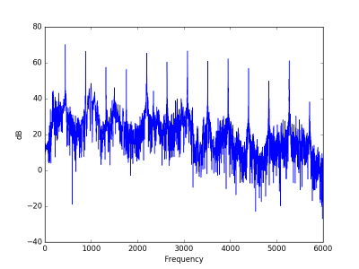
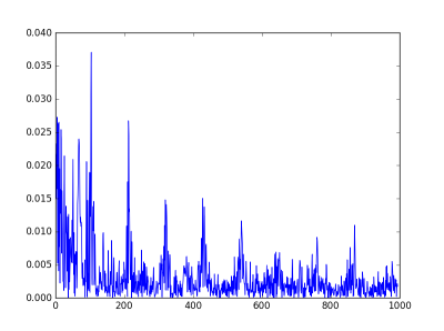
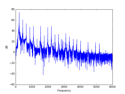
How close is that guess to being correct? It has to be exactly correct when η is 0 or 1, but how well does it do in the middle? Here are a few experiments fixing γ = 1 and varying σ.