Fermat’s factoring trick and cryptography

Many encryption algorithms rely on the difficulty of factoring a large number n. If you want to make n hard to factor, you want it to have only two factors. Otherwise, the more factors n has, the smaller the smallest factor must be.

So if you want n to be the product of two large primes, p and q, you want to pick these primes to be roughly the same size so that the smaller factor is as large as possible. If you’re limited on the size of n, then you want p and q to be roughly of size √n. But not too close to √n. You may see in a description of a cryptographic algorithm, such as RSA, “Pick two large primes p and q, but not too close together, …” Why is that?

The answer goes back to Fermat (1607–1665). His factoring trick is to start with an odd composite n and look for numbers a and b such that

n = a² – b²

because if you can do that, then

n = (ab)(a – b).

This trick always works [1], but it’s only practical when the factors are close together. If they are close together, you can do a brute force search for a and b. But otherwise you’re better off doing something else.

Small example

To give an example, suppose we want to factor n = 12319. Then √n = 110.99, so we can start looking for a and b by trying a = 111. We increment a until a² – n is a square, b².

Now 111² – 12319 = 2, so that didn’t work. But 112² – 12319 = 225, which is a square, and so we take a = 112 and b = 15. This tells us p = 112+15 = 127 and q = 112 – 15 = 97.

Larger example with Python code

Now let’s do a larger example, too big to do by hand and more similar to a real application.

    from sympy import sqrt, log, ceiling, Integer

    def is_square(n):
        return type(sqrt(n)) == Integer

    def fermat_factor(n):
        num_digits = int(log(n, 10).evalf() + 1)
        a = ceiling( sqrt(n).evalf(num_digits) )

        counter = 0
        while not is_square(a*a - n):
            a += 1
            counter += 1

        b = sqrt(a*a - n)
        return(a+b, a-b, counter)

    p = 314159200000000028138418196395985880850000485810513
    q = 314159200000000028138415196395985880850000485810479
    print( fermat_factor(p*q) )

This recovers p and q in 3,580 iterations. Note that the difference in p and q is large in absolute terms, approximately 3 × 1027, but small relative to p and q.

Related posts

[1] If n = pq, then you can set a = (p + q)/2 and b = (p – q)/2.


Empirically testing the Chowla conjecture

Terry Tao’s most recent blog post looks at the Chowla conjecture theoretically. This post looks at the same conjecture empirically using Python. (Which is much easier!)

The Liouville function λ(n) is (-1)Ω(n) where Ω(n) is the number of prime factors of n counted with multiplicity. So, for example, Ω(9) = 2 because even though 9 has only one distinct prime factor, that factor counts twice.

Given some set of k strides h1, h2, …, hk, define

f(n) = λ(n + h1) λ(n + h1) … λ(n + hk).

The Chowla conjecture says that the average of the first N values of f(n) tends to zero as N goes to infinity. This has been proven for k = 1 but not for larger k.

If f(n) acts like a Bernoulli random variable, our experiments might increase our confidence in the conjecture, but they wouldn’t prove anything. Unexpected results wouldn’t prove anything either, but a departure from random behavior might help find a counterexample if the conjecture is false.

We’re going to be evaluating the Liouville function repeatedly at the same arguments, so it will save some compute time if we tabulate its values. This will also let us use some compact Python notation to average f. We’ll need to tabulate the function up to Nhk.

In the code below, maxstride is an upper bound on the strides hk we may look at. SymPy has a function primeomega that calculates Ω(n) so we might as well use it. If you wanted to use a very large value of N, you might want to fill the array of Liouville function values using a more direct approach that avoids all the factoring implicit in calls to primeomega.

    from sympy import primeomega
    from numpy import empty

    N = 10000
    maxstride = 100

    liouville = empty(N + maxstride)
    liouville[0] = 1
    for n in range(1, len(liouville)):
        liouville[n] = (-1)**primeomega(n)

The following code looks at the Chowla conjecture for h1 = 0 and h2 ranging over 1, 2, …, 99.

    average = empty(maxstride-1)
    for s in range(1, maxstride):
        average[s-1] = (liouville[0:N] * liouville[s:N+s]).sum()/N

If the Liouville function is distributed like a random variable taking on -1 and 1 with equal probability, we’d expect the averages to vary like samples form a normal distribution with mean 0 and variance 1/(2N).

    print(average.mean())
    print(average.std())
    print( (2*N)**-0.5 )

This returns

    0.00141
    0.00851
    0.00707

and so the means are indeed near zero, and the standard deviation of the samples is about what we’d expect.

What if we replace Ω(n), the number of prime factors with multiplicity, with ω(n), the number of distinct prime factors? The averages above are still small, but the sample variance is about twice as big as before. I’ve seen this pattern with several different large values of N, so I suspect there’s something going on here.

(I didn’t see a function in SymPy corresponding to ω(n), but you can create your own with len(factorint(n)).

Predicting when an RNG will output a given value

A few days ago I wrote about how to pick the seed of a simple random number generator so that a desired output came n values later. The number n was fixed and we varied the seed. In this post, the seed will be fixed and we’ll solve for n. In other words, we ask when a pseudorandom sequence will produce a given value.

In principle you could just run the RNG until you get the output you’re looking for, but we’ll assume such a brute force approach is not feasible or at least not fast enough.

If a LCG (linear congruential generator) has seed z, multiplier a, and modulus m, then the nth output is an z reduced mod m. So our task is to solve

x = an z mod m

for n. If we forget for a moment that we’re working with integers mod m, we see that the solution is

n = loga (x / z)

We can actually make this work if we interpret division by z to mean multiplication by the inverse of z mod m and if we interpret the logarithm to be a discrete logarithm. For more on discrete logarithms and one algorithm for computing them, see this post.

In an earlier post I used  a = 742938285 and m = 231 – 1 = 2147483647. We set n = 100 and solved for z to make the 100th output equal to 20170816, the date of that post. It turned out that z = 1898888478.

Now let’s set the seed z = 1898888478 and ask when the LCG sequence will take on the value x = 20170816. Of course we know that n will turn out to be 100, but let’s pretend we don’t know that. We’ll write a little Python script to find n.

I expect there’s a simple way to compute modular inverses using SymPy, but I haven’t found it, so I used some code from StackOverflow.

The following Python code produces n = 100, as expected.

from sympy.ntheory import discrete_log

def egcd(a, b):
    if a == 0:
        return (b, 0, 1)
    else:
        g, y, x = egcd(b % a, a)
        return (g, x - (b // a) * y, y)

def modinv(a, m):
    g, x, y = egcd(a, m)
    if g != 1:
        raise Exception('modular inverse does not exist')
    else:
        return x % m

a = 742938285
z = 1898888478
m = 2**31 - 1
x = 20170816
zinv = modinv(z, m)

n = discrete_log(m, x*zinv, a)
print(n)

Inverse Fibonacci numbers

As with the previous post, this post is a spinoff of a blog post by Brian Hayes. He considers the problem of determining whether a number n is a Fibonacci number and links to a paper by Gessel that gives a very simple solution: A positive integer n is a Fibonacci number if and only if either 5n2 – 4 or 5n2 + 4 is a perfect square.

If we know n is a Fibonacci number, how can we tell which one it is? That is, if n = Fm, how can we find m?

For large m, Fm is approximately φm / √ 5 and the error decreases exponentially with m. By taking logs, we can solve for m and round the result to the nearest integer.

We can illustrate this with SymPy. First, let’s get a Fibonacci number.

      >>> from sympy import *
      >>> F = fibonacci(100)
      >>> F
      354224848179261915075

Now let’s forget that we know F is a Fibonacci number and test whether it is one.

      >>> sqrt(5*F**2 - 4)
      sqrt(627376215338105766356982006981782561278121)

Apparently 5F2 – 4 is not a perfect square. Now let’s try 5F2 + 4.

      >>> sqrt(5*F**2 + 4)
      792070839848372253127

Bingo! Now that we know it’s a Fibonacci number, which one is it?

      >>> N((0.5*log(5) + log(F))/log(GoldenRatio), 10)
      100.0000000

So F must be the 100th Fibonacci number.

It looks like our approximation gave an exact result, but if we ask for more precision we see that it did not.

      >>> N((0.5*log(5) + log(F))/log(GoldenRatio), 50)
      99.999999999999999999999999999999999999999996687654

Related posts

Three proofs that 2017 is prime

Aaron Meurer asked on Twitter whether there’s a proof that 2017 is prime that would fit into 140 characters.

My first reply was this:

sqrt(2017) < 45.
2017 not divisible by 2, 3, 5, 7, 11, 13, 17, 19, 23, 29, 31, 37, 41, or 43.
Ergo prime.

I’m not sure that’s what he had in mind. There’s some implied calculation (which I didn’t actually do), so it’s kinda cheating. It would be interesting if there were something special about 2017 that would allow a more transparent proof.

(Implicit in the proof above is the theorem that if a number has a prime factor, it has a prime factor less than it’s square root. If you multiply together numbers bigger than the square root of n, you get a product bigger than n.)

Then for fun I gave two more proofs that are more sophisticated but would require far too much work to actually carry out by hand.

The first uses Fermat’s little theorem:

For 0 < a < 2017, a2016 – 1 is divisible by 2017.
2017 is not one of the three Carmichael numbers < 2465.
Ergo prime.

Fermat’s little theorem says that if p is prime, then for any 0 < ap, ap – 1 – 1 is divisible by p. This is actually an efficient way to prove that a number is not prime. Find a number a such that the result doesn’t hold, and you’ve proved that p isn’t prime. For small numbers, the easiest way to show a number is not prime is to show its factors. But for very large numbers, such as those used in cryptography, it’s efficient to have a way to prove that a number has factors without having to actually produce those factors.

Unfortunately, Fermat’s little theorem gives a necessary condition for a number to be prime, but not a sufficient condition. It can appear to be prime for every witness (the bases a are called witnesses) and still not be a prime. The Carmichael numbers pass the Fermat primailty test without being prime. The first four are 561, 1105, 1729, and 2465.

For more on using Fermat’s little theorem to test for primality, see Probability that a number is prime.

The final proof was this:

2016! + 1 is divisible by 2017, and so by Wilson’s theorem 2017 is prime.

Unlike Fermat’s little theorem, Wilson’s theorem gives necessary and sufficient conditions for a number to be prime. A number n is prime if and only if (n-1)! + 1 is divisible by n. In theory you could use Wilson’s theorem to test whether a number is prime, but this would be horrendously inefficient. 2016! has 5,789 digits. (You can find out how many digits n! has without computing it using a trick described here.)

Despite its inefficiency, you can actually use Wilson’s theorem and SymPy to prove that 2017 is prime.

      >>> from sympy import factorial
      >>> x = factorial(2016) + 1
      >>> x % 2017
      0


Prime factors, phone numbers, and the normal distribution

Telephone numbers typically have around three distinct prime factors.

The length of a phone number varies by country, but US a phone number is a 10 digit number, and 10-digit numbers are often divisible by three different prime numbers, give or take a couple. Assuming phone numbers are scattered among possible 10-digit numbers in a way that doesn’t bias their number of prime factors, these numbers will often have between 1 and 5 prime factors. If a country has 9- or 11-digit phone numbers, the result is essentially the same.

Let ω(n) be the number of distinct prime factors of n. Then the Erdős–Kac theorem says roughly that ω(n) is distributed like a normal random variable with mean and variance log log n. More precisely, fix two numbers a and b.  For a given value of x, count the proportion of positive integers less than x where

(ω(n) – log log n) / sqrt( log log n)

is between a and b. Then in the limit as x goes to infinity, this proportion approaches the probability that a standard normal random variable is between a and b.

So by that heuristic, the number of distinct prime factors of a 10-digit number is approximately normally distributed with mean and variance log log 10^11 = 3.232, and such a distribution is between 1 and 5 around 73% of the time.

My business phone number, for example, is 8324228646. Obviously this is divisible by 2. In fact it equals 2 × 32 × 462457147, and so it has exactly three distinct prime factors: 2, 3, and 462457147.

Here’s how you could play with this using Python.

    from sympy.ntheory import factorint

    def omega(n):
        return len(factorint(n))

I looked in SymPy and didn’t see an implementation of ω(n) directly, but it does have a function factorint that returns the prime factors of a number, along with their multiplicities, in a dictionary. So ω(n) is just the size of that dictionary.

I took the first 20 phone numbers in my contacts and ran them through omega and got results consistent with what you’d expect from the theory above. One was prime, and none had more than five factors.

Bar chart of umber of prime factors in a sample of phone numbers with heights [1, 3, 5, 8, 3]

Chi-square goodness of fit test example with primes

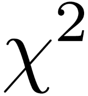
chi squared

Yesterday Brian Hayes wrote a post about the distribution of primes. He showed how you could take the remainder when primes are divided by 7 and produce something that looks like rolls of six-sided dice. Here we apply the chi-square goodness of fit test to show that the rolls are too evenly distributed to mimic randomness. This post does not assume you’ve seen the chi-square test before, so it serves as an introduction to this goodness of fit test.

In Brian Hayes’ post, he looks at the remainder when consecutive primes are divided by 7, starting with 11. Why 11? Because it’s the smallest prime bigger than 7. Since no prime is divisible by any other prime, all the primes after 7 will have a remainder of between 1 and 6 inclusive when divided by 7. So the results are analogous to rolling six-sided dice.

The following Python code looks at prime remainders and (pseudo)random rolls of dice and computes the chi-square statistic for both.

First, we import some functions we’ll need.

    from sympy import prime
    from random import random
    from math import ceil

The function prime takes an argument n and returns the nth prime. The function random produces a pseudorandom number between 0 and 1. The ceiling function ceil rounds its argument up to an integer. We’ll use it to convert the output of random into dice rolls.

In this example we’ll use six-sided dice, but you could change num_sides to simulate other kinds of dice. With six-sided dice, we divide by 7, and we start our primes with the fifth prime, 11.

    num_sides = 6
    modulus = num_sides + 1

    # Find the index of the smallest prime bigger than num_sides
    index = 1
    while prime(index) <= modulus:
        index += 1

We’re going to take a million samples and count how many times we see 1, 2, …, 6. We’ll keep track of our results in an array of length 7, wasting a little bit of space since the 0th slot will always be 0. (Because the remainder when dividing a prime by a smaller number is always positive.)

    # Number of samples
    N = 1000000
    
    observed_primes = [0]*modulus
    observed_random = [0]*modulus

Next we “roll” our dice two ways, using prime remainders and using a pseudorandom number generator.

    for i in range(index, N+index):
        m = prime(i) % modulus
        observed_primes[m] += 1
        m = int(ceil(random()*num_sides))
        observed_random[m] += 1

The chi-square goodness of fit test depends on the observed number of events in each cell and the expected number. We expect 1/6th of the rolls to land in cell 1, 2, …, 6 for both the primes and the random numbers. But in a general application of the chi-square test, you could have a different expected number of observations in each cell.

    expected = [N/num_sides for i in range(1, modulus)]

The chi-square test statistic sums (O – E)2/E over all cells, where O stands for “observed” and E stands for “expected.”

    def chisq_stat(O, E):
        return sum( (o - e)**2/e for (o, e) in zip(O, E) )

Finally, we compute the chi-square statistic for both methods.

    ch = chisq_stat(observed_primes[1:], expected[1:])
    print(ch)

    ch = chisq_stat(observed_random[1:], expected[1:])
    print(ch)

Note that we chop off the first element of the observed and expected lists to get rid of the 0th element that we didn’t use.

When I ran this I got 0.01865 for the prime method and 5.0243 for the random method. Your results for the prime method should be the same, though you might have a different result for the random method.

Now, how do we interpret these results? Since we have six possible outcomes, our test statistics has a chi-square distribution with five degrees of freedom. It’s one less than the number of possibilities because the total counts have to sum to N; if you know how many times 1, 2, 3, 4, and 5 came up, you can calculate how many times 6 came up.

A chi-square distribution with ν degrees of freedom has expected value ν. In our case, we expect a value around 5, and so the chi-square value of 5.0243 is unremarkable. But the value of 0.01864 is remarkably small. A large chi-square statistics would indicate a poor fit, the observed numbers being suspiciously far from their expected values. But a small chi-square value suggests the fit is suspiciously good, closer to the expected values than we’d expect of a random process.

We can be precise about how common or unusual a chi-square statistic is by computing the probability that a sample from the chi square distribution would be larger or smaller. The cdf gives the probability of seeing a value this small or smaller, i.e. a fit this good or better. The sf gives the probability of seeing a value this larger or larger, i.e. a fit this bad or worse. (The scipy library uses sf for “survival function,” another name for the ccdf, complementary cumulative distribution function).

    from scipy.stats import chi2
    print(chi2.cdf(ch, num_sides-1), chi2.sf(ch, num_sides-1))

This says that for the random rolls, there’s about a 41% chance of seeing a better fit and a 59% chance of seeing a worse fit. Unremarkable.

But it says there’s only a 2.5 in a million chance of seeing a better fit than we get with prime numbers. The fit is suspiciously good. In a sense this is not surprising: prime numbers are not random! And yet in another sense it is surprising since there’s a heuristic that says primes act like random numbers unless there’s a good reason why in some context they don’t. This departure from randomness is the subject of research published just this year.

If you look at dice with 4 or 12 sides, you get a suspiciously good fit, but not as suspicious as with 6 sides. But with 8 or 20-sided dice you get a very bad fit, so bad that its probability underflows to 0. This is because the corresponding moduli, 9 and 21, are composite, which means some of the cells in our chi-square test will have no observations. (Suppose m has a proper factor a. Then if a prime p were congruent to a mod m, p would be have to be divisible by a.)

Update: See the next post for a systematic look at different moduli.

You don’t have to use “dice” that correspond to regular solids. You could consider 10-sided “dice,” for example. For such numbers it may be easier to think of spinners than dice, a spinner with 10 equal arc segments it could fall into.

Related post: Probability that a number is prime

Alternating sums of factorials

Richard Guy’s Strong Law of Small Numbers says

There aren’t enough small numbers to meet the many demands made of them.

In his article by the same name [1] Guy illustrates his law with several examples of patterns that hold for small numbers but eventually fail. One of these examples is

3! – 2! + 1! = 5

4! – 3! + 2! – 1! = 19

5! – 4! + 3! – 2! + 1! = 101

6! – 5! + 4! – 3! + 2! – 1! = 619

7! – 6! + 5! – 4! + 3! – 2! + 1! = 4421

8! – 7! + 6! – 5! + 4! – 3! + 2! – 1! = 35899

If we let f(n) be the alternating factorial sum starting with nf(n) is prime for n = 3, 4, 5, 6, 7, 8, but not for n = 9. So the alternating sums aren’t all prime. Is f(n) usually prime? f(10) is, so maybe 9 is the odd one. Let’s write a code to find out.

    from sympy import factorial, isprime

    def altfact(n):
        sign = 1
        sum = 0
        while n > 0:
            sum += sign*factorial(n)
            sign *= -1
            n -= 1
        return sum

    numprimes = 0
    for i in range(3, 1000):
        if isprime( altfact(i) ):
            print(i)
            numprimes += 1
    print(numprimes)

You could speed up this code by noticing that

    altfact(n+1) = factorial(n+1) - altfact(n)

and tabulating the values of altfact. The code above corresponds directly to the math, though it takes a little while to run.

So it turns out the alternating factorial sum is only prime for 15 values less than 1000. In addition to the values of n mentioned above, the other values are 15, 19, 41, 59, 61, 105, 160, and 601.

* * *

[1] The Strong Law of Small Numbers, Richard K. Guy, The American Mathematical Monthly, Vol. 95, No. 8 (Oct., 1988), pp. 697-712.

Last digits of Fibonacci numbers

If you write out a sequence of Fibonacci numbers, you can see that the last digits repeat every 60 numbers.

The 61st Fibonacci number is 2504730781961. The 62nd is 4052739537881. Since these end in 1 and 1, the 63rd Fibonacci number must end in 2, etc. and so the pattern starts over.

It’s not obvious that the cycle should have length 60, but it is fairly easy to see that there must be a cycle. There are only 10*10 possibilities for two consecutive digits. Since the Fibonacci numbers are determined by a two-term recurrence, and since the last digit of a sum is determined by the sum of the last digits, the sequence of last digits must repeat eventually. Here “eventually” means after at most 10*10 terms.

Replace “10” by any other base in the paragraph above to show that the sequence of last digits must be cyclic in any base. In base 16, for example, the period is 24. In hexadecimal notation the 25th Fibonacci number is 12511 and the 26th is 1DA31, so the 27th must end in 2, etc.

Here’s a little Python code to find the period of the last digits of Fibonacci numbers working in any base b.

from sympy import fibonacci as f

def period(b):
    for i in range(1, b*b+1):
        if f(i)%b == 0 and f(i+1)%b == 1:
            return(i)

This shows that in base 100 the period is 300. So in base 10 the last two digits repeat every 300 terms.

The period seems to vary erratically with base as shown in the graph below.

Related: Applied number theory

Numerators of harmonic numbers

Harmonic numbers

The nth harmonic number, Hn, is the sum of the reciprocals of the integers up to and including n. For example,

H4 = 1 + 1/2 + 1/3 + 1/4 = 25/12.

Here’s a curious fact about harmonic numbers, known as Wolstenholme’s theorem:

For a prime p > 3, the numerator of Hp-1 is divisible by p2.

The example above shows this for p = 5. In that case, the numerator is not just divisible by p2, it is p2, though this doesn’t hold in general. For example, H10 = 7381/2520. The numerator 7381 is divisible by 112 = 121, but it’s not equal to 121.

Generalized harmonic numbers

The generalized harmonic numbers Hn,m are the sums of the reciprocals of the first n positive integers, each raised to the power m. Wolstenholme’s theorem also says something about these numbers too:

For a prime p > 3, the numerator of Hp-1,2 is divisible by p.

For example, H4,2 = 205/144, and the numerator is clearly divisible by 5.

Computing with Python

You can play with harmonic numbers and generalized harmonic numbers in Python using SymPy. Start with the import statement

from sympy.functions.combinatorial.numbers import harmonic

Then you can get the nth harmonic number with harmonic(n) and generalized harmonic numbers with harmonic(n, m).

To extract the numerators, you can use the method as_numer_denom to turn the fractions into (numerator, denominator) pairs. For example, you can create a list of the numerators of the first 10 harmonic numbers with

[harmonic(n).as_numer_denom()[0] for n in range(10)]

What about 0?

You might notice that harmonic(0) returns 0, as it should. The sum defining the harmonic numbers is empty in this case, and empty sums are defined to be zero.