Scott Hanselman has a good article on freeing up disk space under Windows Vista. I tried one of his suggestions and immediately freed up seven GB on my wife’s PC.
Month: October 2008
What happens when you add a new teller?

Suppose a small bank has only one teller. Customers take an average of 10 minutes to serve and they arrive at the rate of 5.8 per hour. What will the expected waiting time be? What happens if you add another teller?
We assume customer arrivals and customer service times are random (details later). With only one teller, customers will have to wait nearly five hours on average before they are served. But if you add a second teller, the average waiting time is not just cut in half; it goes down to about 3 minutes. The waiting time is reduced by a factor of 93x.
Why was the wait so long with one teller? There’s not much slack in the system. Customers are arriving every 10.3 minutes on average and are taking 10 minutes to serve on average. If customer arrivals were exactly evenly spaced and each took exactly 10 minutes to serve, there would be no problem. Each customer would be served before the next arrived. No waiting.
The service and arrival times have to be very close to their average values to avoid a line, but that’s not likely. On average there will be a long line, 28 people. But with a second teller, it’s not likely that even two people will arrive before one of the tellers is free.
Here are the technical footnotes. This problem is a typical example from queuing theory. Customer arrivals are modeled as a Poisson process with λ = 5.8/hour. Customer service times are assumed to be exponential with mean 10 minutes. (The Poisson and exponential distribution assumptions are common in queuing theory. They simplify the calculations, but they’re also realistic for many situations.) The waiting times given above assume the model has approached its steady state. That is, the bank has been open long enough for the line to reach a sort of equilibrium.
Queuing theory is fun because it is often possible to come up with surprising but useful results with simple equations. For example, for a single server queue, the expected waiting time is λ/(μ(μ – λ)) where λ the arrival rate and μ is the service rate. In our example, λ = 5.8 per hour and μ = 6 per hour. Some applications require more complicated models that do not yield such simple results, but even then the simplest model may be a useful first approximation.
Update: More details and equations here. Non-technical overview of queueing theory here.
Related links
Data synthesis
This post makes a good point: what we call data analysis would be called data synthesis if stuck to the ordinary meanings of the words.
Via Andrew Gelman.
Nearly everyone is above average
Most people have a higher than average number of legs.
The vast majority of people have two legs. But some people have no legs or one leg. So the average number of legs will be just slightly less than 2, meaning most people have an above average number of legs. (I didn’t come up with this illustration, but I can’t remember where I saw it.)
Except in Lake Wobegon, it’s not possible for everyone to be above average. But this example shows it is possible for nearly everyone to be above average. And when you’re counting numbers of social connections, nearly everyone is below average. What’s not possible is for a majority of folks to be above or below the median.
Most people expect half the population to be above and below average in every context. This is because they confuse mean and median. And even among people who understand the difference between mean and median, there is a strong tendency to implicitly assume symmetry. And when distributions are symmetric, the mean and the median are the same.
Comparing two ways to fit a line to data
Suppose you have a set of points and you want to fit a straight line to the data. I’ll present two ways of doing this, one that works better numerically than the other.
Given points (x1, y1), …, (xN, yN) we want to fit the best line of the form y = mx + b, best in the sense of minimizing the square of the differences between the actual data yi values and the predicted values mxi + b.
The textbook solution is the following sequence of equations.
The equations above are absolutely correct, but turning them directly into software isn’t the best approach. Given vectors of x and y values, here is C++ code to compute the slope m and the intercept b directly from the equations above.
	double sx = 0.0, sy = 0.0, sxx = 0.0, sxy = 0.0;
	int n = x.size();
	for (int i = 0; i < n; ++i)
	{
		sx += x[i];
		sy += y[i];
		sxx += x[i]*x[i];
		sxy += x[i]*y[i];
	}
	double delta = n*sxx - sx*sx;
	double slope = (n*sxy - sx*sy)/delta;
	double intercept = (sxx*sy - sx*sxy)/delta;
This direct method often works. However, it presents multiple opportunities for loss of precision. First of all, the Δ term is the same calculation criticized in this post on computing standard deviation. If the x values are large relative to their variance, the Δ term can be inaccurate, possibly wildly inaccurate.
The problem with computing Δ directly is that it could potentially require subtracting nearly equal numbers. You always want to avoid computing a small number as the difference of two big numbers if you can. The equations for slope and intercept have a similar vulnerability.
The second method is algebraically equivalent to the method above, but it is better suited to numerical calculation. Here it is in code.
	double sx = 0.0, sy = 0.0, stt = 0.0, sts = 0.0;
	int n = x.size();
	for (int i = 0; i < n; ++i)
	{
		sx += x[i];
		sy += y[i];
	}
	for (int i = 0; i < n; ++i)
	{
		double t = x[i] - sx/n;
		stt += t*t;
		sts += t*y[i];
	}

	double slope = sts/stt;
	double intercept = (sy - sx*slope)/n;
This method involves subtraction, and it too can fail for some data sets. But in general it does better than the former method.
Here are a couple examples to show how the latter method can succeed when the former method fails.
First we populate x and y as follows.
	for (int i = 0; i < numSamples; ++i)
	{
		x[i] = 1e10 + i;
		y[i] = 3*x[i] + 1e10 + 100*GetNormal();
	}
Here GetNormal() is generator for standard normal random variables. Aside from some small change due to the random noise, we would expect slope 3 and intercept 1010.
The most direct method gives slope -0.666667 and intercept 5.15396e+10. The better method gives slope: 3.01055 and intercept: 9.8945e+9. If we remove the Gaussian noise and try again, the direct method gives slope 3.33333 and intercept 5.72662e+9 while the better method is exactly correct: slope 3 intercept and 1e+10.
As another example, fill x and y as follows.
	for (int i = 0; i < numSamples; ++i)
	{
		x[i] = 1e6*i;
		y[i] = 1e6*x[i] + 50 + GetNormal();
	}
Now both method compute the intercept exactly as 1e6 but the direct method computes the intercept as 60.0686 while the second method computes 52.416. Neither is very close to the theoretical value of 50, but the latter method is closer.
To read more about why one way can be so much better than the other, see this writeup on the analogous issue with computing standard deviation: theoretical explanation for numerical results.
Update: See related post on computing correlation coefficients.
Networks and power laws
In many networks—social networks, electrical power networks, networks of web pages, etc.—the number of connections for each node follows a statistical distribution known as a power law. Here’s a model of network formation that shows how power laws can emerge from very simple rules.
Albert-László Barabási describes the following algorithm in his book Linked. Create a network by starting with two connected nodes. Then add nodes one at a time. Every time a new node joins the network, it connects to two older nodes at random with probability proportional to the number of links the old nodes have. That is, nodes that already have more links are more likely to get new links. If a node has three times as many links as another node, then it’s three times as attractive to new nodes. The rich get richer, just like with Page Rank.
Barabási says this algorithm produces networks whose connectivity distribution follows a power law. That is, the number of nodes with n connections is proportional to n–k. In particular he says k = 3.
I wrote some code to play with this algorithm. As the saying goes, programming is understanding. There were aspects of the algorithm I never would have noticed had I not written code for it. For one thing, after I decided to write a program I had to read the description more carefully and I noticed I’d misunderstood a couple details.
If the number of nodes with n connections really is proportional to n–k, then when you plot the number of nodes with 1, 2, 3, … connections, the points should fall near a straight line when plotted on the log-log scale and the slope of this line should be –k.
In my experiment with 10,000 nodes, I got a line of slope -2.72 with a standard error of 0.04. Not exactly -3, but maybe the theoretical result only holds in the limit as the network becomes infinitely large. The points definitely fall near a straight line in log-log scale: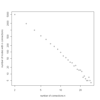
In this example, about half the nodes (5,073 out of 10,000) had only two connections. The average number of connections was 4, but the most connected node had 200 connections.
Note that the number of connections per node does not follow a bell curve at all. The standard deviation on the number of connections per node was 6.2. This means the node with 200 connections was over 30 standard deviations from the average. That simply does not happen with normal (Gaussian) distributions. But it’s not unusual at all for power law distributions because they have such thick tails.
Of course real networks are more complex than the model given here. For example, nodes add links over time, not just when they join a network. Barabási discusses in his book how some elaborations of the original model still produce power laws (possibly with different exponents) and while others do not.
42nd Carnival of Mathematics hosted here soon
There was some confusion over when and where the next Carnival of Mathematics will be hosted. It will be here on Friday, October 24. Please help spread the word since the date is earlier than the originally announced date.
Please submit your best recent math posts via the Blog Carnival site.
A few previous Carnivals of Mathematics: 41, 40, 39
Table-driven text munging in PowerShell
In my previous post, I mentioned formatting C++ code as HTML by doing some regular expression substitutions. I often need to write something that carries out a list of pattern substitutions, so I decided to rewrite the previous script to read a list of patterns from a file. Another advantage of putting the list of substitutions in an external file is that the same file could be used from scripts written in other languages.
Here’s the code:
param($regex_file)

$lines = get-content $regex_file

$a = get-clipboard

foreach( $line in $lines )
{
    $line = ($line.trim() -replace "s+", " ")
    $pair = $line.split(" ", [StringSplitOptions]::RemoveEmptyEntries)
    $a = $a -replace $pair
}

out-clipboard $a
The part of the script that is unique to formatting C++ as HTML is moved to a separate file, say cpp2html.txt, that is pass in as an argument to the script.
& & < < > > " " ' '
Now I could use the same PowerShell script for any sort of task that boils down to a list of pattern replacements. (Often this kind of rough translation does not have to be done perfectly. It only has to be done well enough to reduce the amount of left over manual work to an acceptable level. You start with a small list of patterns and add more patterns until it’s less work to do the remaining work by hand than to make the script smarter.)
Note that the order of the lines in the file can be important. Substitutions are done from the top of the list down. In the example above, we want to first convert & to & then convert < to <. Otherwise, < would first become < and then become &lt;.
Manipulating the clipboard with PowerShell
The PowerShell Community Extensions contain a couple handy cmdlets for working with the Windows clipboard: Get-Clipboard and Out-Clipboard. One way to use these cmdlets is to copy some text to the clipboard, munge it, and paste it somewhere else. This lets you avoid creating a temporary file just to run a script on it.
Update: Looks like
For example, occasionally I need to copy some C++ source code and paste it into HTML in a <pre> block. While <pre> turns off normal HTML formatting, special characters still need to be escaped: < and > need to be turned into < and > etc. I can copy the code from Visual Studio, run a script html.ps1 from PowerShell, and paste the code into my HTML editor. (I like to use Expression Web.)
The script html.ps1 looks like this.
$a = get-clipboard;
$a = $a -replace "&", "&";
$a = $a -replace "<", "<";
$a = $a -replace ">", ">";
$a = $a -replace '"', """
$a = $a -replace "'", "'"
out-clipboard $a
So this C++ code
    double& x = y;
    char c = 'k';
    string foo = "hello";
    if (p < q) ...
turns into this HTML code
    double& x = y;
    char c = 'k';
    string foo = "hello";
    if (p < q) ...
Of course the PSCX clipboard cmdlets are useful for more than HTML encoding. For example, I wrote a post a few months ago about using them for a similar text manipulation problem.
If you’re going to do much text manipulation, you may want to look at these notes on regular expressions in PowerShell.
The only problem I’ve had with the PSCX clipboard cmdlets is copying formatted text. The cmdlets work as expected when copying plain text. But here’s what I got when I copied the word “snippets” from the CodeProject home page and ran Get-Clipboard:
    Version:0.9
    StartHTML:00000136
    EndHTML:00000214
    StartFragment:00000170
    EndFragment:00000178
    SourceURL:https://www.codeproject.com/
    <html><body>
    <!--StartFragment-->snippets<!--EndFragment-->
    </body>
    </html>
The Get-Clipboard cmdlet has a -Text option that you might think would copy content as text, but as far as I can tell the option does nothing. This may be addressed in a future release of PSCX.
Default arguments and lazy evaluation in R
In C++, default function arguments must be constants, but in R they can be much more general. For example, consider this R function definition.
f <- function(a, b=log(a)) { a*b }
If f is called with two arguments, it returns their product. If f is called with one argument, the second argument defaults to the logarithm of the first. That’s convenient, but it gets more surprising. Look at this variation.
f <- function(a, b=c) {c = log(a); a*b}
Now the default argument is a variable that doesn’t exist until the body of the function executes! If f is called with one argument, the R interpreter chugs along until it gets to the last line of the function and says “Hmm. What is b? Let me go back and see. Oh, the default value of b is c, and now I know what c is.”
This behavior is called lazy evaluation. Expressions are not evaluated unless and until they are needed. It’s a common feature of functional programming languages.
There’s a little bit of lazy evaluation in many languages: the second argument of a Boolean expression is often not evaluated if the expression value is determined by the first argument. For example, the function bar() in the expression
while (foo() && bar())
will not be called if the function foo() returns false. But functional languages like R take lazy evaluation much further.
R was influenced by Scheme, though you could use R for a long time without noticing its functional roots. That speaks well of the language. Many people find functional programming too hard and will not use languages that beat you over the head with their functional flavor. But it’s intriguing to know that the functional capabilities are there in case they’re needed.