I spoke with Sacha Chua last week. We talked about entrepreneurship, Emacs, having eclectic interests, delegation, and more.
J: I ran into you by searching on Emacs topics. When I look at your blog, I see that you do a lot of interesting things, but it’s a little hard to get a handle on exactly what you do.
S: Oh, the dreaded networking quirky question. What exactly do you do?
J: Yeah, people have said the same thing to me. Not to put you in a box, but I was curious. I see from your site that you do graphic art—sketching and such—and it doesn’t create the impression that you’re someone who would spend a lot of time in front of Emacs. So I’m curious how these things fit together, how you got started using Emacs and how you use it now.
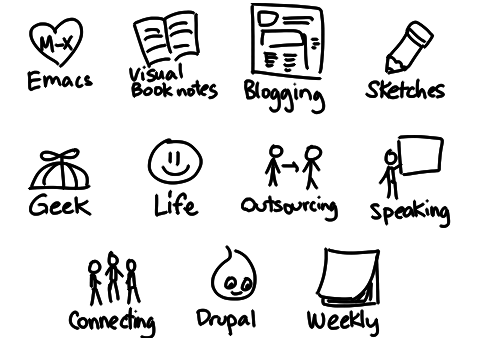
S: So my background is actually fairly technical. I’ve been doing computer programming for ages and ages. In high school I came across a book Unix Power Tools, which is how I got interested in Emacs. And because I was interested in programming, in open source, a little bit of wearable computing as well, I got to know Emacs and all these different modules it had. For example, Emacspeak is amazing! It’s been around since the 1990s and it’s a great way to use the computer while you’re walking around. Because I love programming and because I wanted to find a way to help out, I ended up maintaining PlannerMode and later EmacsWiki mode as well.
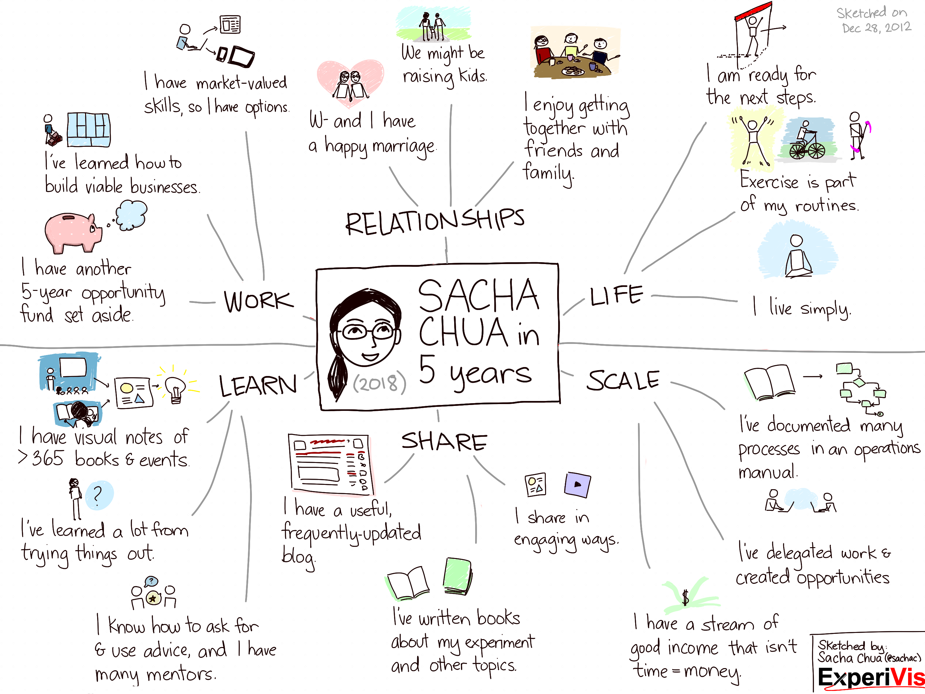
When I went to university, I took up computer science. After I finished, I taught. Then I took my masters in Toronto, where I am now. Emacs was super helpfu;—being able to do everything in one place. After I finished my masters, I did a lot of software consulting with IBM. I did business consulting as well. Then in 2012, after saving up, I decided to go on pretty much the same adventure you’re on. I’m completely unhirable for the next five years! Most businesses struggle for the first five years, so I saved up enough to not worry too much about my expenses for the next five years. I’m one year in, four years to go, and that’s where I am.
At networking events, I like to shake people up a bit by telling them I’m semi-retired. I’m in this five-year experiment to see how awesome life can be and what I can do to make things better. I’ve done technical consulting, business consulting, sketching, illustration, writing, all sorts of things. Basically, my job description is context-dependent.
J: I understand that.
S: I use Emacs across all the things I do. When I’m doing technical and business consulting, I use Emacs to edit code, to draft documents, even to outline comic strips. And when I’m doing illustration, Emacs—especially Org Mode—helps me keep track of clients and deliverables, things to do, agenda, calendar, deadlines.
J: I’m basically running my life through Org Mode right now. When you say you use Emacs to draft documents, are you using LaTeX?
S: I used LaTeX when I was working on my master’s thesis and other papers, I think. Now I mostly use org mode and export from there.
J: Are you using Emacs for email?
S: I used to. But I’m stuck on Windows to use drawing programs like Sketchbook Pro on my Tablet PC. So it’s harder to set up my email like I had it set up when I used Ubuntu. Back when I used Ubuntu, I was very happy with Gnus.
J: Do you work entirely on Windows, or do you go back and forth between operating systems?
S: I have a private server that runs Linux. On Windows I run Cygwin, but I miss some of the conveniences I had when I had a nicely set-up Linux installation.
J: When you’re running Emacs on Windows, I’m sure you run into things that don’t quite work. What do you do about that?
S: Most things work OK if they’re just Emacs Lisp, but some things call a shell command or use some library that hasn’t been ported over yet. Then I basically wail and gnash my teeth. Sometimes I get things working by using Cygwin, but sometimes it’s a bit of a mess. I don’t use Emacs under Cygwin because I prefer how it works natively. I don’t run into much that doesn’t work.
J: So what programming languages do you use when you’re writing code?
S: I do a lot of quick-and-dirty things in Emacs Lisp. When I need to do some XML parsing or web development, I’ll use Ruby because a lot of people can read it and there are a lot of useful gems. Sometimes I’ll do some miscellaneous things in Perl.
I love doing programming and putting together tools. And I quite enjoy drawing, helping people with presentation and design. So this is left brain plus right brain.
It does boggle people that you can have more than one passion, but others are, like, “Yeah, I know, I’m like that too.”
J: I think having an interest in multiple things is a healthier lifestyle, but it’s a little harder to market.
S: Actually, no. I finally figured out a name for my company, ExperiVis, after a year of playing with it. People reach out to me and we figure out whether it’s a good fit. I don’t need to necessarily guide people to just this aspect or another of my work. I like the fact that people bump into these different things.
J: When we scheduled this call, I went through your virtual assistant. How do you use a virtual assistant?
S: One of the things I don’t like to do is scheduling. I used to get stressed out about scheduling when I did it myself. I’ve always been interested in delegating and taking advantage of what other people enjoy and are good at. I work with an assistant—Criselda. She lives in the Philippines. I found her on oDesk. She works one to four hours a week, more or less, and keeps track of her time.
J: What else might you ask a VA to do?
S: I’ve asked people to do web research. I’ve had someone do a little bit of illustration for me. I’ve had someone do a little bit of programming for me because I want to learn how to delegate technical tasks. He does some Rails prototyping for me. I have someone doing data entry and transcription. It’s fascinating to see how you can swap money for time, especially for things that stress me out, or bore me, or things I can’t do.
Every week I go over my task list with my VA to see which of the tasks I should have delegated. Still working on it!
* * *
Later on in the conversation Sacha asked about my new career and had this gem of advice:
Treating this as a grand experiment makes it much easier for me to try different approaches and not be so scared, to not treat it as a personal rejection if something doesn’t work.
Related post: People I’ve interviewed and people who have interviewed me