The previous post discussed fitting an ellipse and a parabola to the same data. Both fit well, but the ellipse fit a little better. This will often be the case because an ellipse has one more degree of freedom than a parabola.
There is one way to fit a parabola to an ellipse at an extreme point: match the end points and the curvatures. This uses up all the degrees of freedom in the parabola.
When you take the analogous approach to fitting an ellipse to a parabola, you have one degree of freedom left over. The curvature depends on a ratio, and so you can adjust the parameters while maintaining the ratio. You can use this freedom to fit the ellipse better over an interval while still matching the curvature at the vertex.
The rest of the post will illustrate the ideas outlined above.
Fitting a parabola to an ellipse
Suppose you have an ellipse with equation
(x/a)² + (y/b)² = 1.
The curvature at (±a, 0) equals a/b² and the curvature at (0, ±b) equals b/a².
Now if you have a parabola
x = cy² + d
then its curvature at y = 0 is 2|c|.
If you want to match the parabola and the ellipse at (a, 0) then d = a.
To match the curvatures at (a, 0) we set a/b² = 2|c|. So c = −a/2b². (Without the negative sign the curvatures would match, but the parabola would turn away from the ellipse.)
Similarly, at (−a, 0) we have d = −a and c = a/2b². And at (0, ±b) we have d = ±b and c = ∓b/2a².
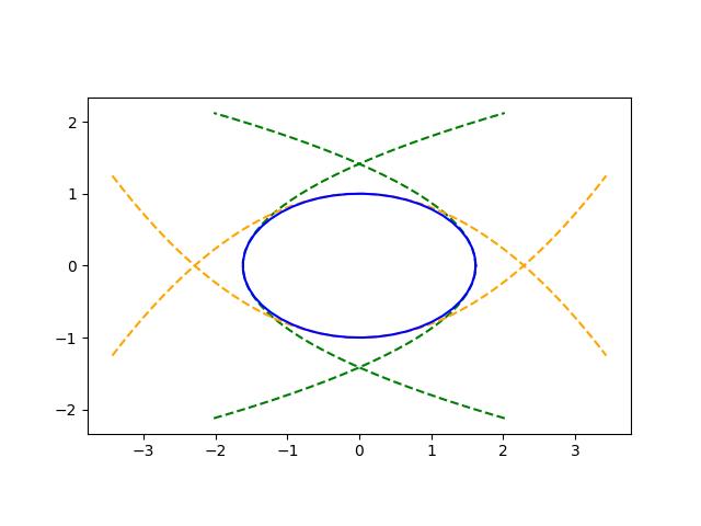
Here’s an example with a golden ellipse.
Fitting an ellipse to a parabola
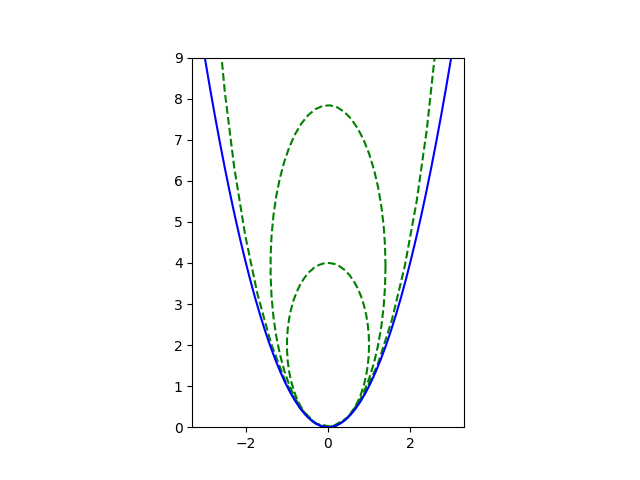
Now we fix the parabola, say
y = cx²
and find an ellipse
(x/a)² + ((y − y0)/b)² = 1
to fit at the vertex (0, 0). For the ellipse to touch the parabola at its vertex we must have
((0 − y0)/b)² = 1
and so y0 = b. To match curvature we have
b/2a² = c.
So a and b are not uniquely determined, only the ratio b/a². As long as this ratio stays fixed at 2c, every ellipse will touch at the vertex and match curvature there. But larger values of the parameters will match the parabola more closely over a wider range. In the limit as b → ∞ (keeping b/a² = 2c), the ellipses become a parabola.