The two previous posts looked at adjacency networks. The first used examples of US states and Texas counties. The second post made suggestions for using these networks in a classroom. This post is a continuation of the previous post using examples from Japan.
Japan is divided into 8 regions and 47 prefectures. Here is a network diagram of the prefectures in the Kanto region showing which regions border each other. (In this post, “border” will be regions share a large enough border that I was able to see the border region on the map I was using. Some regions may share a very small border that I left out.)
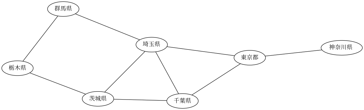
This is a good example of why it is convenient in GraphViz to use variable names that are different from labels. I created my graphs using English versions of prefecture names, and checked my work using the English names. Then after debugging my work I changed the label names (but not the connectivity data) to use Japanese names.
To show what this looks like, my GraphViz started out like this
    graph G {
    layout=sfdp
    AI [label="Aichi"]
    AK [label="Akita"]
    AO [label="Aomori"]
    ...
    AO -- AK
    AO -- IW
    AK -- IW
    ...
and ended up like this
    graph G {
    layout=sfdp
    AI [label="愛知県"]
    AK [label="秋田県"]
    AO [label="青森県"]
    ...
    AO -- AK
    AO -- IW
    AK -- IW
    ...
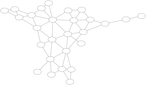
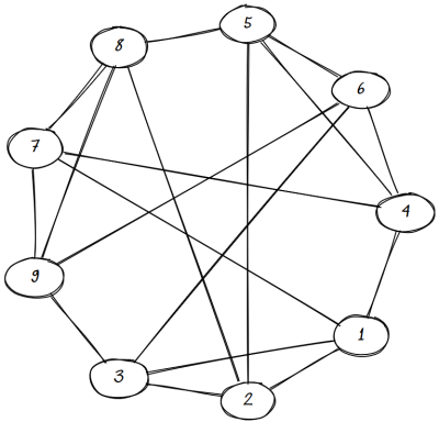
Here’s a graph only showing which prefectures border each other within a region.

This image is an SVG, so you can rescale it without losing any resolution. Here’s the same image as a PDF.
Because this network is effectively several small networks, it would be easy to look at a map and figure out which nodes correspond to which prefectures. (It would be even easier if you could read the labels!)
Note that there are two islands—literal islands, as well as figurative islands in the image above—Hokkaido, which is its own region, and Okinawa, which a prefecture in the Kyushu region.
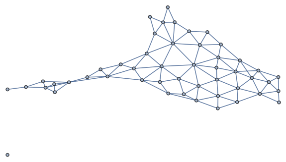
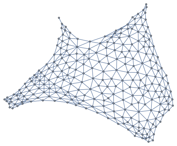
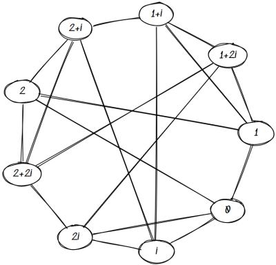
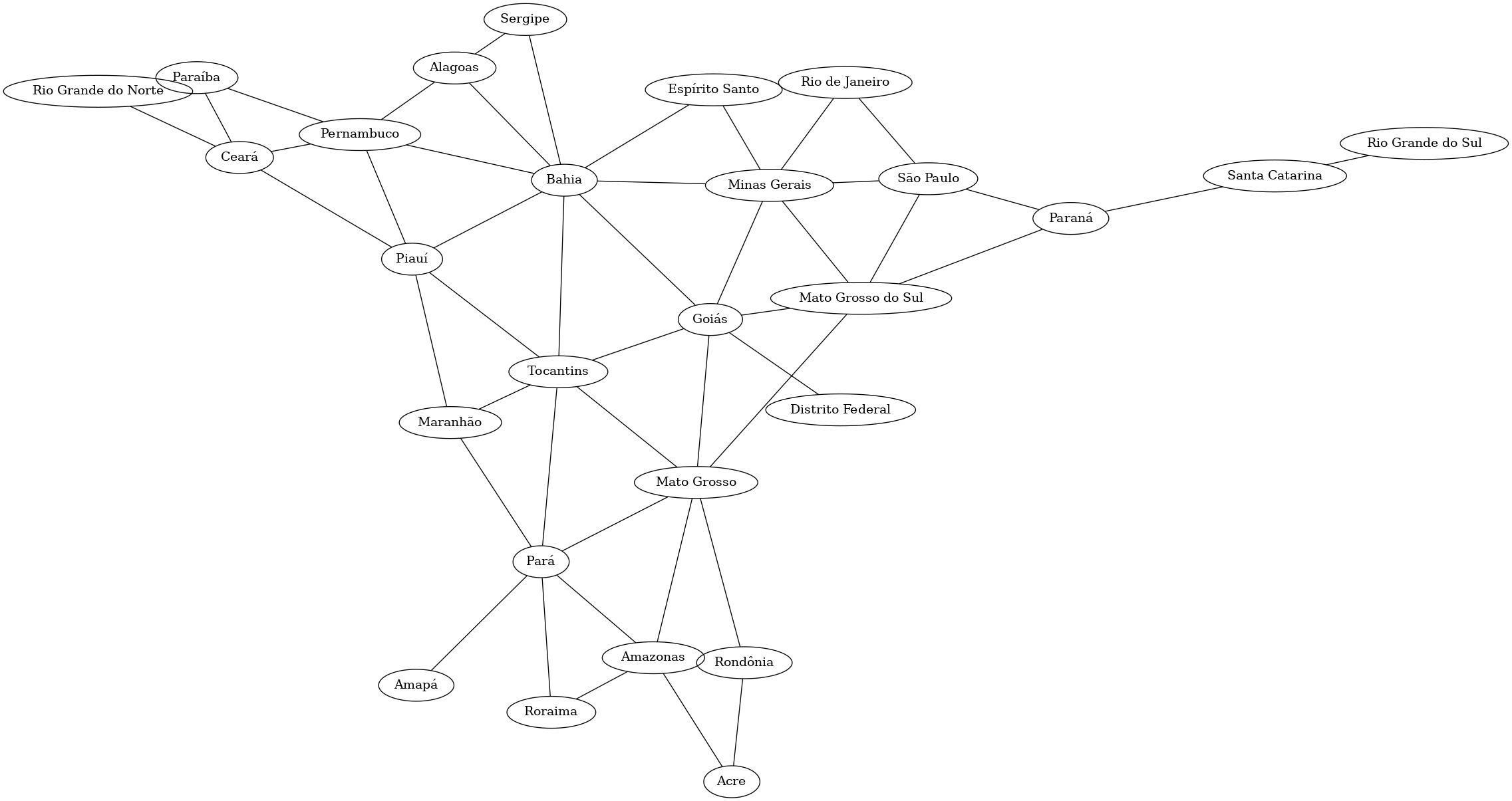
Here’s the graph with all bordering relations, including across regions.

The image above is also an SVG. And here’s the same image as a PDF.