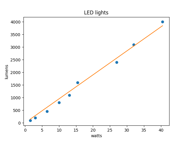
Posts tagged as:

Probability and Statistics

Probability approximations

by John on June 22, 2008

When I took my first probability course, it seemed like there were an infinite number of approximation theorems to learn, all mysterious. Looking back, there were probably only two or three, and they don’t need to be mysterious.

For example, under the right circumstances you can approximate a Binomial(n, p) well with a Normal(np, np(1-p)). While the relationship between the parameters in these two distributions is obvious to the initiated, it’s not at all obvious to a beginner. It seems much clearer to say that a Binomial can be approximated by a Normal with the same mean and variance. After all, a distribution that doesn’t get the mean and variance correct doesn’t sound like a very promising approximation.

Taking it a step further, a good teacher could guide a class to discover this approximation themselves. This would take more time than simply stating the result and working an example or two, but the difference in understanding would be immense. And if you’re not going to take the time to aim for understanding, what’s the point in covering approximation theorems at all? They’re not used that often for computation anymore. In my opinion, the only reason to go over them is the insight they provide.

{ 0 comments }

Today I talked to a doctor about the design of a randomized clinical trial that would use a Bayesian monitoring rule. The probability of response on each arm would be modeled as a binomial with a beta prior. Simple conjugate model. The historical response rate in this disease is only 5%, and so the doctor had chosen a beta(0.1, 1.9) prior so that the prior mean matched the historical response rate.

For beta distributions, the sum of the two parameters is called the effective sample size. There is a simple and natural explanation for why a beta(a, b) distribution is said to contain as much information as a+b data observations. By this criterion, the beta(0.1, 1.9) distribution is not very informative: it only has as much influence as two observations. However, viewed in another light, a beta(0.1, 1.9) distribution is highly informative.

This trial was designed to stop when the posterior probability is more than  0.999 that one treatment is more effective than the other. That’s an unusually high standard of evidence for stopping a trial — a cutoff of 0.99 or smaller would be much more common — and yet a trial could stop after only six patients. If X is the probability of response on one arm and Y is the probability of response on the other, after three failures on the first treatment and three successes on the other, Pr(Y > X) > 0.999.

The explanation for how the trial could stop so early is that the prior distribution is, in an odd sense, highly informative. The trial starts with a strong assumption that each treatment is ineffective. This assumption is somewhat justified by of experience, and yet a beta(0.1, 1.9) distribution doesn’t fully capture the investigator’s prior belief.

(Once at least one response has been observed, the beta(0.1, 1.9) prior becomes essentially uninformative. But until then, in this context, the prior is informative.)

A problem with a beta prior is that there is no way to specify the mean at 0.05 without also placing a large proportion of the probability mass below 0.05. The beta prior places too little probability on better outcomes that might reasonably happen. I imagine a more diffuse prior with mode 0.05 rather than mean 0.05 would better describe the prior beliefs regarding the treatments.

The beta prior is convenient because Bayes’ theorem takes a very simple form in this case: starting from a beta(a, b) prior and observing s successes and f failures, the posterior distribution is beta(a+s, b+f).  But a prior less convenient algebraically could be more robust and better adept at representing prior information.

A more basic observation is that “informative” and “uninformative” depend on context. This is part of what motivated Jeffreys to look for prior distributions that were equally (un)informative under a set of transformations. But Jeffreys’ approach isn’t the final answer. As far as I know, there’s no universally acceptable resolution to this dilemma.

{ 1 comment }

Robust priors

by John on June 8, 2008

Yesterday I posted a working paper version of an article I’ve been working on with Jairo Fúquene and Luis Pericchi: A Case for Robust Bayesian priors with Applications to Binary Clinical Trials.

Bayesian analysis begins with a prior distribution, a function summarizing what is believed about an experiment before any data are collected. The prior is updated as data become available and becomes the posterior distribution, a function summarizing what is currently believed in light of the data collected so far. As more data are collected, the relative influence of the prior decreases and the influence of the data increases. Whether a prior is robust depends on the rate at which the influence of the prior decreases.

There are essentially three approaches to how the influence of the prior on the posterior should vary as a function of the data.

  1. Robustness with respect to the prior. When the data and the prior disagree, give more weight to the data.
  2. Conjugate priors. The influence of the prior is independent of the extent to which it agrees with the data.
  3. Robustness with respect to the data. When the data and the prior disagree, give more weight to the prior.

When I say “give more weight to the data” or “give more weight to the prior,” I’m not talking about making ad hoc exceptions to Bayes theorem. The weight given to one or the other falls out of the usual application of Bayes theorem. Roughly speaking, robustness has to do with the relative thickness of the tails of the prior and the likelihood. A model with thicker tails on the prior will be robust with respect to the prior, and a model with thicker tails on the likelihood will be robust with respect to the data.

Each of the three approaches above are appropriate in different circumstances. When priors come from well-understood physical principles, it may make sense to use a model that is robust with respect to the data, i.e. to suppress outliers. When priors are based on vague beliefs, it may make more sense to be robust with respect to the prior. Between these extremes, particularly when a large amount of data is available, conjugate priors may be appropriate.

When the data and the prior are in rough agreement, the contribution of a robust prior to the posterior is comparable to the contribution that a conjugate prior would have had. (And so using robust proper priors leads to greater variance reduction than using improper priors.) But as the level of agreement decreases, the contribution of a robust prior to the posterior also decreases.

In the paper, we show that with a binomial likelihood, the influence of a conjugate prior grows without bound as the prior mean goes to infinity. However, with a Student-t prior, the influence of the prior is bounded as the prior mean increases. For a Cauchy prior, the influence of the prior is bounded as the location parameter goes to infinity.

It’s easy to confuse a robust prior and a vague conjugate prior. Our paper shows how in a certain sense, even an “informative” Cauchy distribution is less informative than a “non-informative” conjugate prior.

{ 1 comment }

I’m teaching part of a basic medical statistics class this summer. It’s been about a decade since I’ve taught basic probability and statistics and I now have different ideas about what is important. For example, I now think it’s more important that a beginning class understand the law of small numbers than the law of large numbers.

One reason for my change of heart is that over the intervening years I’ve talked with people who have had a class like the one I’m teaching now and I have some idea what they got out of it. They might summarize their course as follows.

First we did probability. You know, coin flips and poker hands. Then we did statistics. That’s where you look up these numbers in tables and if the number is small enough then what you’re trying to prove is true, and otherwise it’s false.

Too many people get through a course in probability and statistics without understanding what probability has to do with statistics. I think we’d be better off “covering” far less material but trying to insure that students really grok two or three big ideas by the time they leave.

{ 5 comments }

Barriers to good statistical software

by John on May 16, 2008

I attended a National Cancer Institute workshop yesterday entitled “Barriers to producing well-tested, user-friendly software for cutting-edge statistical methodology.” I was pleased that everyone there realized there is a huge difference between code created for personal use and reliable software that others would willingly use. Not all statisticians appreciate the magnitude of the difference.

I was also pleased that several people at the workshop were aware of the problem of irreproducible statistical analyses. Not everyone was aware how serious or how common the problem is, but those who were aware were adamant that something needs to be done about it, such as journals requiring authors to publish the code used to analyze their data.

{ 3 comments }

Bias

by John on May 7, 2008

An unbiased estimator, very roughly speaking, is a statistic that gives the correct result on average. For a precise definition, see Wikipedia. Unbiasedness is an intuitively desirable property. In fact, it seems indispensable at first.

In the colloquial sense, “bias” is practically synonymous with self-serving dishonesty. Who wants a self-serving, dishonest statistical estimate? But it’s important to remember that “bias” in statistical sense has a technical meaning that may not correspond to the colloquial meaning.

Here’s the big problem with statistical bias: if U is an unbiased estimator of θ, f(U) is NOT an unbiased estimator of f(θ) in general. For example, standard deviation is the square root of variance, but the square root of an unbiased estimator for variance is not an unbiased estimator for standard deviation. This shows bias has nothing to do with accuracy, since the square root of an accurate estimation of variance is an accurate estimate of standard deviation. In fact, unbiased estimators can be terrible.

The fact that unbiasedness is not preserved under transformations calls into question its usefulness. People seldom care directly about abstract statistical parameters directly. Instead they care about some calculation based on those parameters. An unbiased estimate of the parameters does not generally lead to an unbiased estimate of what people really want to estimate.

{ 0 comments }

How to calculate binomial probabilities

by John on April 24, 2008

Suppose you’re doing something that has probability of success p and probability of failure q = 1-p. If you repeat what you’re doing m+n times, the probability of m successes and n failures is given by  

\frac{(m+n)!}{m!\, n!} p^m q^n

Now suppose m and n are moderately large. The terms (m+n)! and m! n! will be huge, but the terms pm and qn will be tiny. The huge terms might overflow, and the tiny terms might underflow, even though the final result may be a moderate-sized number. The numbers m and n don’t have to be that large for this to happen since factorials grow very quickly. On a typical system, overflow happens if m+n > 170. How do you get to the end result without having to deal with impossibly large or small values along the way?

The trick is to work with logs. You want to first calculate log( (m+n)! ) - log( m! ) - log( n! ) + m log( p ) + n log( q ) , then exponentiate the result. This pattern comes up constantly in statistical computing.

Libraries don’t always include functions for evaluating factorial or log factorial. They’re more likely to include functions for Γ(x) and its log. For positive integers n, Γ(n+1) = n!. Now suppose you have a function lgamma that computes log Γ(x). You might write something like this.

    double probability(double p, double q, int m, int n)
    { 
        double temp = lgamma(m + n + 1.0);
        temp -=  lgamma(n + 1.0) + lgamma(m + 1.0);
        temp += m*log(p) + n*log(q);
        return exp(temp);
    }

The function lgamma is not part of the ANSI standard library for C or C++, but it is part of the POSIX standard. On Unix-like systems, lgamma is included in the standard library. However, Microsoft does not include lgamma as part of the Visual C++ standard library. On Windows you have to either implement your own lgamma function or grab an implementation from somewhere like Boost.

Here’s something to watch out for with POSIX math libraries. I believe the POSIX standard does not require a function called gamma for evaluating the gamma function Γ(x). Instead, the standard requires functions lgamma for the log of the gamma function and tgamma for the gamma function itself. (The mnemonic is “t” for “true,” meaning that you really want the gamma function.) I wrote a little code that called gamma and tested it on OS X and Red Hat Linux this evening. In both cases gcc compiled the code without warning, even with the -Wall and -pedantic warning flags. But on the Mac, gamma was interpreted as tgamma and on the Linux box it was interpreted as lgamma. This means that gamma(10.0) would equal 362880 on the former and 12.8018 on the latter.

{ 4 comments }

Four types of errors

by John on April 21, 2008

There are two kinds of errors discussed in classical statistics, unimaginatively named Type I and Type II. Aside from having completely non-mnemonic names, they represent odd concepts.

Technically, a Type I error consists of rejecting the “null hypothesis” (roughly speaking, the assumption of no effect, the hypothesis you typically set out to disprove) in favor of the “alternative hypothesis” when in fact the null hypothesis is true. A Type II error consists of accepting the null hypothesis (technically, failing to reject the null hypothesis) when in fact the null hypothesis is false.

Suppose you’re comparing two treatments with probabilities of efficacy θj and θk. The typical null hypothesis is that θj = θk, i.e. that the treatments are identically effective. The corresponding alternative hypothesis is that θj ≠ θk, that the treatments are not identical. Andrew Gelman says in this presentation (page 87)

I’ve never made a Type 1 error in my life. Type 1 error is θj = θk, but I claim they’re different. I’ve never studied anything where θj = θk.

I’ve never made a Type 2 error in my life. Type 2 error is θj ≠ θk, but I claim they’re the same. I’ve never claimed that θj = θk.

But I make errors all the time!

(Emphasis added.) The point is that no two treatments are ever identical. People don’t usually mean to test whether two treatments are exactly equal but rather that they’re “nearly” equal, though they are often fuzzy about what “nearly” means.

Instead of Type I and Type II errors, Gelman proposes we concentrate on “Type S” errors (sign errors, concluding θj > θk when in fact θj < θk) and “Type M” errors (magnitude errors, concluding that an effect is larger than it truly is.)

{ 0 comments }

Are Covey’s quadrants correlated?

by John on April 8, 2008

I was reading a statistical article the other day that used the word “important” when I thought perhaps they should have said “urgent.” Since I was in a statistical frame of mind, I wondered whether importance and urgency are positively or negatively correlated.

Stephen Covey is known for his four quadrant diagram and his advice that we should spend as much time as we can in quadrant 2, working on things that are important but not urgent.

The four-quadrant matrix for importance and urgency.

Are urgent tasks more likely, less likely, or equally likely to be important? In statistical jargon, are they positively correlated, negatively correlated, or uncorrelated?

I believe Covey’s assumption is that urgency is negatively correlated with importance, that is, urgent tasks are less likely to be important. That’s probably true of life in general, but there are contexts where the correlation is reversed. In the paper that prompted this musing, I believe urgency and importance were positively correlated.

In what areas of life are urgency and importance most positively correlated? Most negatively correlated?

{ 0 comments }

Learning is not the same as just gaining information. Sometimes learning means letting go of previously held beliefs. While this is true in life in general, my point here is to show how this holds true when using the mathematical definition of information.

The information content of a probability density function p(x) is given by

integral of p(x) log p(x)

Suppose we have a Beta(2, 6) prior on the probability of success for a binary outcome.

plot of beta(2,6) density

The prior density has information content 0.597. Then suppose we observe a success. The posterior density is distributed as Beta(3, 6). The posterior density has information 0.516, less information than the prior density.

plot of beta(3,6) density

Observing a success pulled the posterior density toward the right. The posterior density is a little more diffuse than the prior and so has lower information content. In that sense, we know less than before we observed the data! Actually, we’re less certain than we were before observing the data. But if the true probability of response is larger than our prior would indicate, we’re closer to the truth by becoming less confident of our prior belief, and we’ve learned something.

{ 0 comments }

God is in the details

by John on March 30, 2008

Some say “The devil is in the details,” meaning solutions break down when you examine them closely enough. Some say “God is in the details,” meaning opportunities for discovery and creativity come from digging into the details. Both are true, but the latter is more interesting.

I posted something along these lines a few weeks ago, Six quotes on digging deep. In that post I quote Richard Feynman

… nearly everything is really interesting if you go into it deeply enough …

I thought about this again last night when I ran across a post by Andrew Gelman entitled God is in every leaf of every tree. He has a similar quote from Feynman.

No problem is too small or too trivial if we really do something about it.

From there he links to a post where he describes what he calls the paradox of importance. Sometimes we can do our most creative work on the least important problems. The important problems often demand quick solutions, so we fall back on familiar methods.

Everything in this post applies equally well to creativity in other fields: graphic design, music composition, literature, etc.  However, Gelman is talking about creativity specifically in the context of statistics. Statistics is a prime example of something that appears dull from the outside but becomes fascinating in the details. A course in statistics can be mind-numbingly dull when the emphasis is on rote application of black-box procedures. Looking inside the boxes is more interesting, and designing the boxes is most interesting.

{ 0 comments }

Innovation IV

by John on March 26, 2008

John Tukey said

efficiency = statistical efficiency x usage.

I don’t know the context of this quote, but here’s what I think Tukey meant. The usefulness of a statistical method depends not just on the method’s abstract virtues, but also on how often the method can be used and how often in fact it is used. This ties in with Michael Schrage’s comment that innovation is not what innovators do but what customers adopt.

{ 0 comments }

Multiple comparisons

by John on March 21, 2008

Multiple comparisons present a conundrum in classical statistics. The options seem to be:

  1. do nothing and tolerate a high false positive rate
  2. be extremely conservative and tolerate a high false negative rate
  3. do something ad hoc between the extremes

A new paper by Andrew Gelman, Jennifer Hill, and Masanao Yajima opens with “The problem of multiple comparisons can disappear when viewed from a Bayesian perspective.” I would clarify that the resolution comes not from the Bayesian perspective per se but from the Bayesian hierarchical perspective.

See this blog post for a link to the article “Why we (usually) don’t have to worry about multiple comparisons” and to a presentation by the same title.

{ 0 comments }

Plausible reasoning

by John on March 19, 2008

If Socrates is probably a man, he’s probably mortal.

How do you extend classical logic to reason with uncertain propositions, such as the statement above? Suppose we agree to represent degrees of plausibility with real numbers, larger numbers indicating greater plausibility. If we also agree to a few axioms to quantify what we mean by consistency and common sense, there is a unique system that satisfies the axioms. The derivation is tedious and not well suited to a blog posting, so I’ll cut to the chase: given certain axioms, the inevitable system for plausible reasoning is probability theory.

There are two important implications of this result. First, it is possible to develop probability theory with no reference to sets. This renders much of the controversy about the interpretation of probability moot. Instead of arguing about what a probability can and cannot represent, one could concede the point. “We won’t use probabilities to represent uncertain information. We’ll use ‘plausibilities’ instead, derived from rules of common sense reasoning. And by the way, the resulting theory is identical to probability theory.”

The other important implication is that all other systems of plausible reasoning — fuzzy logic, neural networks, artificial intelligence, etc. — must either lead to the same conclusions as probability theory, or violate one of the axioms used to derive probability theory.

See the first two chapters of Probability Theory by E. T. Jaynes for a full development. It’s interesting to note that the seminal paper in this area came out over 60 years ago. (Richard Cox, “Probability, frequency, and reasonable expectation”, 1946.)

{ 1 comment }

Second homes

by John on March 18, 2008

Designing good surveys is hard work. Andrew Gelman posted an example of unintended consequences in survey design yesterday. A survey question asked “How many people do you know who have a second home?” Apparently some respondents thought the question was asking about folks who own vacation homes while others thought the question referred to immigrants.

{ 0 comments }