Check out Seth Godin’s latest post: The uncanny valley.

If you find this photo disturbing, read Seth’s article to see why.
Check out Seth Godin’s latest post: The uncanny valley.
If you find this photo disturbing, read Seth’s article to see why.
This post looks at computing P(X > Y) where X and Y are gamma random variables. These inequalities are central to the Thall-Wooten method of monitoring single-arm clinical trials with time-to-event outcomes. They also are central to adaptively randomized clinical trials with time-to-event outcomes.
When X and Y are gamma random variables P(X > Y) can be computed in terms of the incomplete beta function. Suppose X has shape αX and scale βX and Y has shape αY and scale βY. Then βXY/(βX Y+ βYX) has a beta(αY, αX) distribution. (This result is well-known in the special case of the scale parameters both equal to 1. I wrote up the more general result here but I don’t imagine I was the first to stumble on the generalization.) It follows that
P(X < Y) = P(B < βX/(βX+ βY))
where B is a beta(αY, αX) random variable.
For more details, see Numerical evaluation of gamma inequalities.
Previous posts on random inequalities:
On my other blog, Reproducible Ideas, I wrote two short posts about this morning about reproducibility.
The first post is a pointer to an interview with Roger Barga about Trident, a workflow system for reproducible oceanographic research using Microsoft’s workflow framework.
The second post highlights a paragraph from the interview explaining the idea of provenance in art and scientific research.
If you’ve ever been surprised by a program that printed some cryptic letter combination when you were expecting a number, you’ve run into an arithmetic exception. This article explains what caused your problem and what you may be able to do to fix it.
IEEE floating-point exceptions
Here’s a teaser. If x is of type float or double, does the expression (x == x) always evaluate to true? Are you certain?
Jeremy Freese had an interesting observation about interactions in a recent blog post, responding to a post by Andrew Gelman.
Anything that affects anyone affects different people differently.
Freese was making a point about statistical modeling, but his comment is worth thinking about more generally.
Here’s a summary of the blog posts I’ve written so far regarding PowerShell, grouped by topic.
Three posts announced CodeProject articles related to PowerShell: automated software builds, text reviews for software, and monitoring legacy code.
Three posts on customizing the command prompt: I, II, III.
Two posts on XML sitemaps: making a sitemap and filtering a sitemap.
Two Unix-related posts: cross-platform PowerShell and comparing PowerShell and bash.
The rest of the PowerShell posts I’ve written so far fall under miscellaneous.
Much to my surprise, the post on integer division in PowerShell has been one of the most popular.
It has always seemed odd to me that computer science refers to the number of operations necessary to execute an algorithm as the “complexity” of the algorithm. For example, an algorithm that takes O(N3) operations is more complex than an algorithm that takes O(N2) operations. The big-O analysis of algorithms is important, but “complexity” is the wrong name for it.
Software engineering is primarily concerned with mental complexity, the stress on your brain when working on a piece of code. Mental complexity might be unrelated to big-O complexity. They might even be antithetical: a slow, brute-force algorithm can be much easier to understand that a fast, subtle algorithm.
Of course mental complexity is subjective and hard to measure. The McCabe complexity metric, counting the number of independent paths through a chunk of code, is easy to compute and surprisingly helpful, even though it’s a crude approximation to what you’d really like to measure. (SourceMonitor is a handy program for computing McCabe complexity.)
Kolmogorov complexity is another surrogate for mental complexity. The Kolmogorov complexity of a problem is the length of the shortest computer program that could solve that problem. Kolmogorov complexity is difficult to define precisely — are we talking Java programs? Lisp programs? Turing machines? — and practically impossible to compute, but it’s a useful concept.
I like to think of a variation of Kolmogorov complexity even harder to define, the shortest program that “someone who programs like I do” could write to solve a problem. I started to describe this variation as “impractical,” but in some ways it’s very practical. It’s not practical to compute, but it’s a useful idealization to think about as long as you don’t take it too seriously.
Valen Johnson and I recently posted a working paper on a method for stopping trials of ineffective drugs earlier. For Bayesians, we argue that our method is more consistently Bayesian than other methods in common use. For frequentists, we show that our method has better frequentist operating characteristics than the most commonly used safety monitoring method.
The paper looks at binary and time-to-event trials. The results are most dramatic for the time-to-event analog of the Thall-Simon method, the Thall-Wooten method, as shown below.
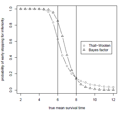
This graph plots the probability of concluding that an experimental treatment is inferior when simulating from true mean survival times ranging from 2 to 12 months. The trial is designed to test a null hypothesis of 6 months mean survival against an alternative hypothesis of 8 months mean survival. When the true mean survival time is less than the alternative hypothesis of 8 months, the Bayes factor design is more likely to stop early. And when the true mean survival time is greater than the alternative hypothesis, the Bayes factor method is less likely to stop early.
The Bayes factor method also outperforms the Thall-Simon method for monitoring single-arm trials with binary outcomes. The Bayes factor method stops more often when it should and less often when it should not. However, the difference in operating characteristics is not as pronounced as in the time-to-event case.
The paper also compares the Bayes factor method to the frequentist mainstay, the Simon two-stage design. Because the Bayes factor method uses continuous monitoring, the method is able to use fewer patients while maintaining the type I and type II error rates of the Simon design as illustrated in the graph below.
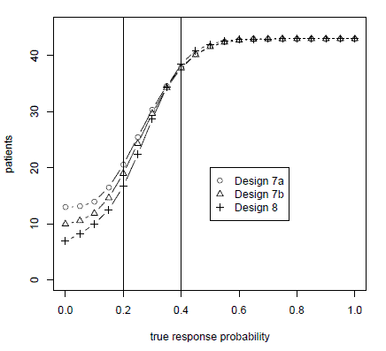
The graph above plots the number of patients used in a trial testing a null hypothesis of a 0.2 response rate against an alternative of a 0.4 response rate. Design 8 is the Bayes factor method advocated in the paper. Designs 7a and 7b are variations on the Simon two-stage design. The horizontal axis gives the true probabilities of response. We simulated true probabilities of response varying from 0 to 1 in increments of 0.05. The vertical axis gives the number of patients treated before the trial was stopped. When the true probability of response is less than the alternative hypothesis, the Bayes factor method treats fewer patients. When the true probability of response is better than the alternative hypothesis, the Bayes factor method treats slightly more patients.
Design 7a is the strict interpretation of the Simon method: one interim look at the data and another analysis at the end of the trial. Design 7b is the Simon method as implemented in practice, stopping when the criteria for continuing cannot be met at the next analysis. (For example, if the design says to stop if there are three or fewer responses out of the first 15 patients, then the method would stop after the 12th patient if there have been no responses.) In either case, the Bayes factor method uses fewer patients. The rejection probability curves, not shown here, show that the Bayes factor method matches (actually, slightly improves upon) the type I and type II error rates for the Simon two-stage design.
Related: Adaptive clinical trial design
When I hear people talking about something growing “exponentially” I think of the line from the Princess Bride where Inigo Montoya says
You keep using that word. I do not think it means what you think it means.
When most people say “exponential” they mean “really fast.” But that’s not what exponential growth means at all. Many things really do grow exponentially (for a while), but not everything that is “really fast” is exponential. Exponential growth can be amazingly fast, but it can also be excruciatingly slow. See Coping with exponential growth.
What does the redirection operator > in PowerShell do to text: leave it as Unicode or convert it to ASCII? The answer depends on whether the thing to the right of the > operator is a file or a program.
Strings inside PowerShell are 16-bit Unicode, instances of .NET’s System.String class. When you redirect the output to a file, the file receives Unicode text. As Bruce Payette says in his book Windows PowerShell in Action,
myScript > file.txtis just syntactic sugar formyScript | out-file -path file.txt
and out-file defaults to Unicode. The advantage of explicitly using out-file is that you can then specify the output format using the -encoding parameter. Possible encoding values include Unicode, UTF8, ASCII, and others.
If the thing on the right side of the redirection operator is a program rather than a file, the encoding is determined by the variable $OutputEncoding. This variable defaults to ASCII encoding because most existing applications do not handle Unicode correctly. However, you can set this variable so PowerShell sends applications Unicode. See Jeffrey Snover’s blog post OuputEncoding to the rescue for details.
Of course if you’re passing strings between pieces of PowerShell code, everything says in Unicode.
Thanks to J_Tom_Moon_79 for suggesting a blog post on this topic.