Mathematical modeling for medical devices

We’re about to see a lot of new, powerful, inexpensive medical devices come out. And to my surprise, I’ve contributed to a few of them.

Growing compute power and shrinking sensors open up possibilities we’re only beginning to explore. Even when the things we want to observe elude direct measurement, we may be able to infer them from other things that we can now measure accurately, inexpensively, and in high volume.

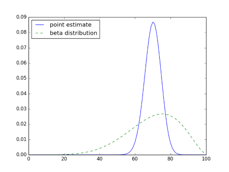
In order to infer what you’d like to measure from what you can measure, you need a mathematical model. Or if you’d like to make predictions about the future from data collected in the past, you need a model. And that’s where I come in. Several companies have hired me to help them create medical devices by working on mathematical models. These might be statistical models, differential equations, or a combination of the two. I can’t say much about the projects I’ve worked on, at least not yet. I hope that I’ll be able to say more once the products come to market.

I started my career doing mathematical modeling (partial differential equations) but wasn’t that interested in statistics or medical applications. Then through an unexpected turn of events, I ended up spending a dozen years working in the biostatistics department of the world’s largest cancer center.

After leaving MD Anderson and starting my consultancy, several companies have approached me for help with mathematical problems associated with their idea for a medical device. These are ideal projects because they combine my earlier experience in mathematical modeling with my more recent experience with medical applications.

If you have an idea for a medical device, or know someone who does, let’s talk. I’d like to help.


Publishable

For an article to be published, it has to be published somewhere. Each journal has a responsibility to select articles relevant to its readership. Articles that make new connections might be unpublishable because they don’t fit into a category. For example, I’ve seen papers rejected by theoretical journals for being too applied, and the same papers rejected by applied journals for being too theoretical.

“A bird may love a fish but where would they build a home together?” — Fiddler on the Roof


One of my favorite proofs: Lagrange multipliers

One of my lightbulb moments in college was when my professor, Jim Vick, explained the Lagrange multiplier theorem. The way I’d seen it stated in a calculus text gave me no feel for why it should be true, but his explanation made sense immediately.

Suppose f(x) is a function of several variables, i.e. x is a vector, and g(x) = c is a constraint. Then the Lagrange multiplier theorem says that at the maximum of f subject to the constraint g we have ∇f = λ ∇g.

Where does this mysterious λ come from? And why should the gradient of your objective function be related to the gradient of a constraint? These seem like two different things that shouldn’t even be comparable.

Here’s the geometric explanation. The set of points satisfying g(x) = c is a surface. And for any k, the set of points satisfying f(x) = k is also surface. Imagine k very large, larger than the maximum of f on the surface defined by g(x) = c. You could think of the surface g(x) = c being a balloon inside the larger balloon  f(x) = k.

Now gradually decrease k, like letting the air out of the outer balloon, until the surfaces g(x) = c and f(x) = k first touch. At that point, the two surfaces will be tangent, and so their normal vectors, given by their gradients, point in the same direction. That is, ∇f and ∇g are parallel, and so ∇f is some multiple of ∇g. Call that multiple λ.

I don’t know how well that explanation works when written down. But when I heard Jim Vick explain it, moving his hands in the air, it was an eye-opener.

This is not a rigorous proof, and it does not give the most general result possible, but it explains what’s going on. It’s something to keep in mind when reading proofs that are more rigorous or more general. As I comment on here,

Proofs serve two main purposes: to establish that a proposition is true, and to show why it is true.

The literally hand-wavy proof scores low on the former criterion and high on the latter.

***

Jim Vick was a great teacher. Some of us affectionately called him The Grinning Demon because he was always smiling, even while he gave devilishly hard homework. He was Dean of Natural Sciences when I took a couple classes from him. He later became Vice President for Student Affairs and kept teaching periodically. He has since retired but still teaches.

After taking his topology course, several of us asked him to teach a differential geometry course. He hesitated because it’s a challenge to put together an undergraduate differential geometry course. The usual development of differential geometry uses so much machinery that it’s typically a graduate-level course.

Vick found a book that starts by looking only at manifolds given by level sets of smooth functions, like the surfaces discussed above. Because these surfaces sit inside a Euclidean space, you can quickly get to some interesting geometric results using elementary methods. We eventually got to the more advanced methods, but by then we had experience in a more tangible setting. As Michael Atiyah said, abstraction should follow experience, not precede it.

Uncertainty in a probability

Suppose you did a pilot study with 10 subjects and found a treatment was effective in 7 out of the 10 subjects.

With no more information than this, what would you estimate the probability to be that the treatment is effective in the next subject? Easy: 0.7.

Now what would you estimate the probability to be that the treatment is effective in the next two subjects? You might say 0.49, and that would be correct if we knew that the probability of response is 0.7. But there’s uncertainty in our estimate. We don’t know that the response rate is 70%, only that we saw a 70% response rate in our small sample.

If the probability of success is p, then the probability of s successes and f failures in the next sf subjects is given by

{s+f \choose s} p^s (1-p)^f

But if our probability of success has some uncertainty and we assume it has a beta(ab) distribution, then the predictive probability of s successes and f failures is given by

{s+f \choose s} \frac{B(a+s, b+f)}{B(a,b)}

where

B(x, y) = \frac{\Gamma(x)\, \Gamma(y)}{\Gamma(x+y)}

In our example, after seeing 7 successes out of 10 subjects, we estimate the probability of success by a beta(7, 3) distribution. Then this says the predictive probability of two successes is approximately 0.51, a little higher than the naive estimate of 0.49. Why is this?

We’re not assuming the probability of success is 0.7, only that the mean of our estimate of the probability is 0.7. The actual probability might be higher or lower. The predictive probability calculates the probability of outcomes under all possible values of the probability, then creates a weighted average, weighing each probability of success by the probability of that value. The differences corresponding to probability above and below 0.7 approximately balance out, but the former carry a little more weight and so we get roughly what we did before.

If this doesn’t seem right, note that mean and median aren’t the same thing for asymmetric distributions. A beta(7,3) distribution has mean 0.7, but it has a probability of 0.537 of being larger than 0.7.

If our initial experiment has shown 70 successes out of 100 instead of 7 out of 10, the predictive probability of two successes would have been 0.492, closer to the value based on point estimate, but still different.

The further we look ahead, the more difference there is between using a point estimate and using a distribution that incorporates our uncertainty. Here are the probabilities for the number of successes out of the next 100 outcomes, using the point estimate 0.3 and using predictive probability with a beta(7,3) distribution.

So if we’re sure that the probability of success is 0.7, we’re pretty confident that out of 100 trials we’ll see between 60 and 80 successes. But if we model our uncertainty in the probability of response, we get quite a bit of uncertainty when we look ahead to the next 100 subjects. Now we can say that the number of responses is likely to be between 30 and 100.

Münchausen numbers

Baron Münchausen

Baron Münchausen

The number 3435 has the following curious property:

3435 = 33 + 44 + 33 + 55.

It is called a Münchausen number, an allusion to fictional Baron Münchausen. When each digit is raised to its own power and summed, you get the original number back. The only other Münchausen number is 1.

At least in base 10. You could look at Münchausen numbers in other bases. If you write out a number n in base b, raise each of its “digits” to its own power, take the sum, and get n back, you have a Münchausen number in base b. For example 28 is a Münchausen number in base 9 because

28ten = 31nine = 33 + 11

Daan van Berkel proved that there are only finitely many Münchausen in any given base. In fact, he shows that a Münchausen number in base b cannot be greater than 2bb, and so you could do a brute-force search to find all the Münchausen numbers in any base.

The upper bound 2bb grows very quickly with b and so brute force becomes impractical for large b. If you wanted to find all the hexadecimal Münchausen numbers you’d have to search 2*1616 = 36,893,488,147,419,103,232 numbers. How could you do this more efficiently?

Beta reduction: The difference typing makes

Beta reduction is essentially function application. If you have a function described by what it does to x and apply it to an argument t, you rewrite the xs as ts. The formal definition of β-reduction is more complicated than this in order to account for free versus bound variables, but this informal description is sufficient for this blog post. We will first show that β-reduction holds some surprises, then explain how these surprises go away when you add typing.

Suppose you have an expression (λx.x + 2)y, which means apply to y the function that takes its argument and adds 2. Then β-reduction rewrites this expression as y + 2. In a more complicated expression, you might be able to apply β-reduction several times. When you do apply β-reduction several times, does the process always stop? And if you apply β-reduction to parts of an expression in a different order, can you get different results?

Failure to normalize

You might reasonably expect that if you apply β-reduction enough times you eventually get an expression you can’t reduce any further. Au contraire!

Consider the expression  (λx.xx) (λx.xx).  Beta reduction says to replace each of the red xs with the expression in blue. But when we do that, we get the original expression (λx.xx) (λx.xx) back. Beta reduction gets stuck in an infinite loop.

Next consider the expression L = (λx.xxy) (λx.xxy). Applying β-reduction the first time gives  (λx.xxy) (λx.xxyy or Ly. Applying β-reduction again yields Lyy. Beta “reduction” doesn’t reduce the expression at all but makes it bigger.

The technical term for what we’ve seen is that β-reduction is not normalizing. A rewrite system is strongly normalizing if applying the rules in any order eventually terminates. It’s weakly normalizing if there’s at least some sequence of applying the rules that terminates. Beta reduction is neither strongly nor weakly normalizing in the context of (untyped) lambda calculus.

Types to the rescue

In simply typed lambda calculus, we assign types to every variable, and functions have to take the right type of argument. This additional structure prevents examples such as those above that fail to normalize. If x is a function that takes an argument of type A and returns an argument of type B then you can’t apply x to itself. This is because x takes something of type A, not something of type function from A to B. You can prove that not only does this rule out specific examples like those above, it rules out all possible examples that would prevent β-reduction from terminating.

To summarize, β-reduction is not normalizing, not even weakly, in the context of untyped lambda calculus, but it is strongly normalizing in the context of simply typed lambda calculus.

Confluence

Although β-reduction is not normalizing for untyped lambda calculus, the Church-Rosser theorem says it is confluent. That is, if an expression P can be transformed by β-reduction two different ways into expressions M and N, then there is an expression T such that both M and N can be reduced to T. This implies that if β-reduction does terminate, then it terminates in a unique expression (up to α-conversion, i.e. renaming bound variables). Simply typed lambda calculus is confluent as well, and so in that context we can say β-reduction always terminates in a unique expression (again up to α-conversion).

Less likely to get half, more likely to get near half

I was catching up on Engines of our Ingenuity episodes this evening when the following line jumped out at me:

If I flip a coin a million times, I’m virtually certain to get 50 percent heads and 50 percent tails.

Depending on how you understand that line, it’s either imprecise or false. The more times you flip the coin, the more likely you are to get nearly half heads and half tails, but the less likely you are to get exactly half of each. I assume Dr. Lienhard knows this and that by “50 percent” he meant “nearly half.”

Let’s make the fuzzy statements above more quantitative. Suppose we flip a coin 2n times for some large number n. Then a calculation using Stirling’s approximation shows that the probability of n heads and n tails is approximately

1/√(πn)

which goes to zero as n goes to infinity. If you flip a coin a million times, there’s less than one chance in a thousand that you’d get exactly half heads.

Next, let’s quantify the statement that nearly half the tosses are likely to be heads. The normal approximation to the binomial tells us that for large n, the number of heads out of 2n tosses is approximately distributed like a normal distribution with the same mean and variance, i.e. mean n and variance n/2. The proportion of heads is thus approximately normal with mean 1/2 and variance 1/8n. This means the standard deviation is 1/√(8n). So, for example, about 95% of the time the proportion of heads will be 1/2 plus or minus 2/√(8n). As n goes to infinity, the width of this interval goes to 0. Alternatively, we could pick some fixed interval around 1/2 and show that the probability of the proportion of heads being outside that interval goes to 0.

Insufficient statistics

Experience with the normal distribution makes people think all distributions have (useful) sufficient statistics [1]. If you have data from a normal distribution, then the sufficient statistics are the sample mean and sample variance. These statistics are “sufficient” in that the entire data set isn’t any more informative than those two statistics. They effectively condense the data for you. (This is conditional on knowing the data come from a normal. More on that shortly.)

With data from other distributions, the mean and variance may not be sufficient statistics, and in fact there may be no (useful) sufficient statistics. The full data set is more informative than any summary of the data. But out of habit people may think that the mean and variance are enough.

Probability distributions are an idealization, of course, and so data never exactly “come from” a distribution. But if you’re satisfied with a distributional idealization of your data, there may be useful sufficient statistics.

Suppose you have data with such large outliers that you seriously doubt that it could be coming from anything appropriately modeled as a normal distribution. You might say the definition of sufficient statistics is wrong, that the full data set tells you something you couldn’t know from the summary statistics. But the sample mean and variance are still sufficient statistics in this case. They really are sufficient, conditional on the normality assumption, which you don’t believe! The cognitive dissonance doesn’t come from the definition of sufficient statistics but from acting on an assumption you believe to be false.

***

[1] Technically every distribution has sufficient statistics, though the sufficient statistic might be the same size as the original data set, in which case the sufficient statistic hasn’t contributed anything useful. Roughly speaking, distributions have useful sufficient statistics if they come from an “exponential family,” a set of distributions whose densities factor a certain way.

Reversing WYSIWYG

The other day I found myself saying that I preferred org-mode files to Jupyter notebooks because with org-mode, what you see is what you get. Then I realized I was using “what you see is what you get” (WYSISYG) in exactly the opposite of the usual sense. Jupyter notebooks are WYSIWYG in the same sense that a Word document is. You work with a nicely formatted file and the changes you make are immediately reflected visually.

The source file for a Jupyter notebook is a JSON document containing formatting instructions, encoded images, and the notebook content. Looking at a notebook file in a text editor is analogous to unzipping a Word document and looking at the XML inside. Here’s a sample:

    "    if (with_grid_):\n",
    "        plt.grid (which=\"both\",ls=\"-\",color=\"0.65\")\n",
    "    plt.show()    "
   ]
  },
  {
   "cell_type": "code",
   "execution_count": 18,
   "metadata": {
    "collapsed": false
   },
   "outputs": [
    {
     "data": {
      "image/png": "iVBORw0KGgoAAAANSUhEUgAAAawAAAESCAYAAA...

It’s hard to diff two Jupyter notebooks because content changes don’t map simply to changes in the underlying file.

We can look a little closer at WYSIWYG and ask what you see where and what you get where. Word documents and Jupyter notebooks are visually WYSIWYG: what you see in the interactive environment (browser) is what you get visually in the final product. Which is very convenient, except for version control and comparing changes.

Org-mode files are functionally WYSIWYG: what you see in the interactive environment (editor) is what you get functionally in the final code.

You could say that HTML and LaTeX are functionally or causally WYSIWYG whereas Word is visually WYSIWYG. Word is visually WYSIWYG in the sense that what you see on your monitor is essentially what you’ll see coming out of a printer. But Word doesn’t always let you see what’s causing your document to look as it does. Why can’t I delete this? Why does it insist on putting that here? HTML and LaTeX work at a lower level, for better and for worse. You may not be able to anticipate how things will look while editing the source, e.g. where a line will break, but cause and effect are transparent.

Everybody wants WYSIWYG, but they have different priorities regarding what they want to see and are concerned about different aspects of what they get.