Sharing secrets using polynomials

This post will present a couple ways to share secrets using polynomials. We have a group of n people who want to share a secret between them so that k of them will have to cooperate in order to unlock the secret. For example, maybe a committee of n = 5 wants to require the cooperation of at least k = 3 members.

Shamir’s method

Adi Shamir came up with the idea of using polynomials to share secrets as follows. First, encode the secret you want to share as an integer a0. Next, generate m = k − 1 other random integers a1 through am and use these as coefficients of a polynomial f of degree m:

f(x) = a_0 + a_1x + a_2x^2 + \cdots + a_mx^m

A trusted party generates n random integer values of x and gives each person an x and the corresponding value of f(x). Since m + 1 points completely determine an mth degree polynomial, if k = m + 1 people share their data, they can recover f, and thus recover the secret number a0. This can be done efficiently, for example, by using Lagrange interpolation. But with fewer than k data points, the polynomial remains undetermined.

In practice we’d work over the integer modulo a large prime p. While fewer than k data points will not let someone completely determine the polynomial f, it will narrow down the possible coefficients if we’re working over the integers. Working modulo a large prime instead reveals less information.

Verifiable secret sharing

There’s a possible problem with Shamir’s method. Maybe the trusted party made a mistake. Or maybe the trusted party was dishonest and shouldn’t have been trusted. How can the parties verify that they have been given valid data without unlocking the secret? Seems we’re at a logical impasse since you’d have to recover the polynomial to know if your points are on the polynomial.

Paul Feldman came up with a way to assure the participants that the secret can be unlocked without giving them the information to unlock it. The trick is to give everyone data that in principle would let them determine the polynomial, but in practice would not.

We choose a large prime p such that p-1 has a large prime factor q [1]. Then the multiplicative group of non-zero integers mod p has a subgroup of order q. Let g be a generator of that group. The idea is to let everyone verify that

y_i = f(x_i)

for their given (xi, yi) by letting them verify that

g^{y_i} = g^{f(x_i)}

where all calculations are carried out mod p. Our trusted party does this by computing

A_i \equiv g^{a_i}\pmod{p}

for each coefficient ai and letting everyone know g and each of the Ai‘s.

In principle, anyone could solve for a0 if they know A0. But in practice, provided q is large enough, this would not be possible because doing so would require solving the discrete logarithm problem, which is computationally difficult. It’s possible to compute discrete logarithms for small q, but the difficulty goes up quickly as q gets larger.

How do the Ai‘s let everyone verify that their (xi, yi) data is correct?

Each person can verify that

g^{y_i} = \prod_{j=0}^m A_j^{x_i^j} 

using the public data and their personal data, and so they can verify that

g^{y_i} = \prod_{j=0}^m A_j^{x_i^j} = \prod_{j=0}^m g^{a_j x_i^j} = g^{f(x_i)} 

Related posts

[1] Conceptually you pick p‘s until you find one so that p − 1 has a large prime factor q. In practice, you’d do it the other way around: search for large primes q until you find one such that, say, 2q + 1 is also prime.

Miscellaneous

Image editor

Image editing software is complicated, and I don’t use it often enough to remember how to do much. I like Paint.NET on Windows because it is in a sort of sweet spot for me, more powerful than Paint and much less complicated than Photoshop.

I found out there’s a program Pinta for Linux that was inspired by Paint.NET. (Pinta runs on Windows, Mac, and BDS as well.)

Exponential sum of the day

I have a page that draws a different image every day, based on putting the month, day, and the laws two digits of the year into an exponential sum. This year’s images have been more intricate than last year’s because 19 is prime.

I liked today’s image.

exponential sum for 2019-02-27

The page has a link to details explaining the equation behind the image, and an animate link to let you see the sequence in which the points are traversed.

Podcast interview

Rebecca Herold posted a new episode of her podcast yesterday in which she asks me questions about privacy and artificial intelligence. [link went away]

Entropy update

I updated my blog post on solving for probability from entropy because Sjoerd Visscher pointed out that a crude approximation I used could be made much more accurate with a minor tweak.

As a bonus, the new error plot looks cool.

approximation error on log scale
Newsletter

My monthly newsletter comes out tomorrow. This newsletter highlights the most popular blog posts of the month.

I used to say something each month about what I’m up to. Then I stopped because it got to be repetitive. Tomorrow I include a few words about projects I have coming up.

The letter S

I was helping my daughter with physics homework last night and she said “Why do they use s for arc length?!” I said that I don’t know, but that it is conventional.

By the way, this section heading is a reference to Donald Knuth’s essay The Letter S where he writes in delightful Knuthian detail about the design of the letter S in TeX. You can find the essay in his book Literate Programming.

What sticks in your head

This morning I read an article by Dennis Felsing about his impressive/intimidating Linux desktop setup. He uses a lot of tools that are not the easiest way to get things done immediately but are long-term productivity investments.

Remembrance of syntax past

Felsing apparently is able to remember the syntax of scores of tools and programming languages. I cannot. Part of the reason is practice. I cannot remember the syntax of any software I don’t use regularly. It’s tempting to say that’s the end of the story: use it or lose it. Everybody has their set of things they use regularly and remember.

But I don’t think that’s all. I remember bits of math that I haven’t used in 30 years. Math fits in my head and sticks. Presumably software syntax sticks in the heads of people who use a lot of software tools.

There is some software syntax I can remember, however, and that’s software closely related to math. As I commented here, it was easy to come back to Mathematica and LaTeX after not using them for a few years.

Imprinting

Imprinting has something to do with this too: it’s easier to remember what we learn when we’re young. Felsing says he started using Linux in 2006, and his site says he graduated college in 2012, so presumably he was a high school or college student when he learned Linux.

When I was a student, my software world consisted primarily of Unix, Emacs, LaTeX, and Mathematica. These are all tools that I quit using for a few years, later came back to, and use today. I probably remember LaTeX and Mathematica syntax in part because I used it when I was a student. (I also think Mathematica in particular has an internal consistency that makes its syntax easier to remember.)

Picking your memory battles

I see the value in Felsing’s choice of tools. For example, the xmonad window manager. I’ve tried it, and I could imagine that it would make you more productive if you mastered it. But I don’t see myself mastering it.

I’ve learned a few tools with lots of arbitrary syntax, e.g. Emacs. But since I don’t have a prodigious memory for such things, I have to limit the number of tools I try to keep loaded in memory. Other things I load as needed, such as a language a client wants me to use that I haven’t used in a while.

Revisiting a piece of math doesn’t feel to me like revisiting a programming language. Brushing up on something from differential equations, for example, feels like pulling a book off a mental shelf. Brushing up on C# feels like driving to a storage unit, bringing back an old couch, and struggling to cram it in the door.

Middle ground

There are things you use so often that you remember their syntax without trying. And there are things you may never use again, and it’s not worth memorizing their syntax just in case. Some things in the middle, things you don’t use often enough to naturally remember, but often enough that you’d like to deliberately remember them. Some of these are what I call bicycle skills, things that you can’t learn just-in-time. For things in this middle ground, you might try something like Anki, a flashcard program with spaced repetition.

However, this middle ground should be very narrow, at least in my experience/opinion. For the most part, if you don’t use something often enough to keep it loaded in memory, I’d say either let it go or practice using it regularly.

Related posts

Testing for primes less than a quintillion

The most common way to test whether a large number is prime is the Miller-Rabin test. If the test says a number is composite, it’s definitely composite. Otherwise the number is very likely, but not certain, to be prime. A pseudoprime is a composite number that slips past the Miller-Rabin test. (Actually, a strong pseudoprime. More on that below.)

Miller-Rabin test

The Miller-Rabin test is actually a sequence of tests, one for each prime number. First you run the test associated with 2, then the test associated with 3, then the one associated with 5, etc. If we knew the smallest numbers for which these tests fail, then for smaller numbers we know for certain that they’re prime if they pass. In other words, we can turn the Miller-Rabin test for probable primes into test for provable primes.

Lower bound on failure

A recent result by Yupeng Jiang and Yingpu Deng finds the smallest number for which the Miller-Rabin test fails for the first nine primes. This number is

N = 3,825,123,056,546,413,051

or more than 3.8 quintillion. So if a number passes the first nine Miller-Rabin tests, and it’s less than N, then it’s prime. Not just a probable prime, but definitely prime. For a number n < N, this will be more efficient than running previously known deterministic primality tests on n.

Python implementation

Let’s play with this in Python. The SymPy library implements the Miller-Rabin test in a function mr.

The following shows that N is composite, and that it is a false positive for the first nine Miller-Rabin tests.

    from sympy.ntheory.primetest import mr

    N = 3825123056546413051
    assert(N == 149491*747451*34233211)
    ps = [2, 3, 5, 7, 11, 13, 17, 19, 23]
    print( mr(N, ps) )

This doesn’t prove that N is the smallest number with these properties; we need the proof of Jiang and Deng for that. But assuming their result is right, here’s an efficient deterministic primality test that works for all n less than N.

    def is_prime(n):
        N = 3825123056546413051
        assert(n < N)
        ps = [2, 3, 5, 7, 11, 13, 17, 19, 23]
        return mr(n, ps)

Jiang and Deng assert that N is also the smallest composite number to slip by the first 10 and 11 Miller-Rabin tests. We can show that N is indeed a strong pseudoprime for the 10th and 11th primes, but not for the 12th prime.

    print( mr(N, [29, 31]) )
    print( mr(N, [37]) )

This code prints True for the first test and False for the second. That is, N is a strong pseudoprime for bases 29 and 31, but not for 37.

Pseudoprimes and strong pseudoprimes

Fermat’s little theorem says that if n is prime, then

an−1 = 1 mod n

for all 0 < an.  This gives a necessary but not sufficient test for primality. A (Fermat) pseudoprime for base a is a composite number n such that the above holds, an example of where the test is not sufficient.

The Miller-Rabin test refines Fermat’s test by looking at additional necessary conditions for a number being prime. Often a composite number will fail one of these conditions, but not always. The composite numbers that slip by are called strong pseudoprimes or sometimes Miller-Rabin pseudoprimes.

Miller and Rabin’s extra testing starts by factoring n-1 into 2sd where d is odd. If n is prime, then for all 0 < a < n either

ad = 1 mod n

or

a2kd = −1 mod n

for all k satisfying 0 ≤ k < s. If one of these two conditions holds for a particular a, then n passes the Miller-Rabin test for the base a.

It wouldn’t be hard to write your own implementation of the Miller-Rabin test. You’d need a way to work with large integers and to compute modular exponents, both of which are included in Python without having to use SymPy.

Example

561 is a pseudoprime for base 2. In fact, 561 is a pseudoprime for every base relatively prime to 561, i.e. it’s a Carmichael number. But it is not a strong pseudoprime for 2 because 560 = 16 × 35, so d = 35 and

235 = 263 mod 561,

which is not congruent to 1 or to -1. In Python,

    
    >>> pow(2, 560, 561)
    1
    >>> pow(2, 35, 561)
    263

More on factoring and finding primes

The point at infinity

As I explained in an earlier post, a first pass at the definition of an elliptic curve is the set of points satisfying

y² = x³ + ax + b.

There are a few things missing from this definition, as indicated before, one being the mysterious “point at infinity.” I gave a hand-waving explanation that you could get rid of this exceptional point by adding an additional coordinate. Here I’ll describe that in more detail.

Projective coordinates

You could add another coordinate z that’s a sort of silent partner to x and y most of the time. Instead of pairs of points (x, y), we consider equivalence classes of points (x, y, z) where two points are equivalent if each is a non-zero multiple of the other [1]. It’s conventional to use the notation (x : y : z) to denote the equivalence class of (x, y, z).

In this construction, the equation of an elliptic curve is

y²z = x³ + axz² + bz³.

Since triples are in the same equivalence class if each is a multiple of the other, we can usually set z equal to 1 and identify the pair (x, y) with (x : y : 1). The “point at infinity” corresponds to the equivalence class (0 : 1 : 0).

NB: A finite projective plane has multiple points at infinity, but only one is on our curve.

Programming hack

From a programming perspective, you could think of z as a finiteness flag, a bit that is set to indicate that the other two coordinates can be taken at face value.

Projective space

This three-coordinate version is called projective coordinates. Textbooks usually start out by defining projective space and then say that an elliptic curve is a set of points in this space. But if you’re focused on the elliptic curve itself, you can often avoid thinking of the projective space it sits in.

One way to think of projective space is that we add a dimension, the extra coordinate, then subtract a dimension by taking equivalence classes. By doing so we almost end up back where we started, but not quite. We have a slightly larger space that includes “points at infinity,” one of which will be on our curve.

Alternating tools

It’s inconvenient to carry around an extra coordinate that mostly does nothing. But it’s also inconvenient to have a mysterious extra point. So which is better? Much of the time you can ignore both the point at infinity and the extra coordinate. When you can’t, you have a choice which way you’d rather think of things. The point at infinity may be easier to think about conceptually, and projective coordinates may be better for doing proofs.

Concrete example

Let’s get concrete. We’ll look at the curve

y² = x³ + x + 1

over the integers mod 5. There are nine points on this curve: (0, ±1), (2, ±1), (3, ±1), (4, ±2), and ∞. (You could replace -1 with 4 and -2 with 3 if you’d like since we’re working mod 5.)

In the three-coordinate version, the points are (0 : ±1 : 1), (2 : ±1 : 1), (3 : ±1 : 1), (4 : ±2 : 1), and (0 : 1 : 0).

Related posts

[1] We leave out (0, 0, 0). It doesn’t exist in the world we’re constructing, i.e. projective space.

More of everything

If you want your music to have more bass, more mid-range, and more treble, then you just want the music louder. You can increase all three components in absolute terms, but not in relative terms. You can’t increase the proportions of everything.

Would you like more students to major in STEM subjects? OK, what subjects would you like fewer students to major in? English, perhaps? Administrators are applauded when they say they’d like to see more STEM majors, but they know better than to say which majors they’d like to see fewer of.

We have a hard time with constraints.

I’m all for win-win, make-the-pie-bigger solutions when they’re possible. And often they are. But sometimes they’re not.

Regression, modular arithmetic, and PQC

Linear regression

Suppose you have a linear regression with a couple predictors and no intercept term:

β1x1 + β2x2 = y + ε

where the x‘s are inputs, the β are fixed but unknown, y is the output, and ε is random error.

Given n observations (x1, x2, y + ε), linear regression estimates the parameters β1 and β2.

I haven’t said, but I implicitly assumed all the above numbers are real. Of course they’re real. It would be strange if they weren’t!

Learning with errors

Well, we’re about to do something strange. We’re going to pick a prime number p and do our calculations modulo p except for the addition of the error ε. Our inputs (x1, x2) are going to be pairs of integers. Someone is going to compute

r = β1x1 + β2x2 mod p

where β1 and β2 are secret integers. Then they’re going to tell us

r/p + ε

where ε is a random variable on the interval [0, 1].  We give them n pairs (x1, x2) and they give back n values of r/p with noise added. Our job is to infer the βs.

This problem is called learning with errors or LWE. It’s like linear regression, but much harder when the problem size is bigger. Instead of just two inputs, we could have m inputs with m secret coefficients where m is large. Depending on the number of variables m, the number of equations n, the modulus p, and the probability distribution on ε, the problem may be possible to solve but computationally very difficult.

Why is it so difficult? Working mod p is discontinuous. A little bit of error might completely change our estimation of the solution. If n is large enough, we could recover the coefficients anyway, using something like least squares. But how would we carry that out? If m and p are small we can just try all pm possibilities, but that’s not going to be practical if m and p are large.

In linear regression, we assume there is some (approximately) linear process out in the real world that we’re allowed to reserve with limited accuracy. Nobody is playing a game with us, that is just how data come to us. But with LWE, we are playing a game that someone has designed to be hard. Why? For cryptography. In particular, quantum-resistant cryptography.

Post Quantum Cryptography

Variations on LWE are the basis for several proposed encryption algorithms that believed to be secure even if an adversary has access to a quantum computer.

The public key encryption systems in common use today would all be breakable if quantum computing becomes practical. They depend on mathematical problems like factoring and discrete logarithms being computationally difficult, which they appear to be with traditional computing resources. But we know that these problems could be solved in polynomial time on a quantum computer with Shor’s algorithm. But LWE is a hard problem, even on a quantum computer. Or so we suspect.

The US government’s National Institute of Standards and Technology (NIST) is holding a competition to identify quantum-resistant encryption algorithms. Last month they announced 26 algorithms that made it to the second round. Many of these algorithms depend on LWE or variations.

One variation is LWR (learning with rounding) which uses rounding rather than adding random noise. There are also ring-based counterparts RLWE and RLWR which add random errors and use rounding respectively. And there are polynomial variations such as poly-LWE which uses a polynomial-based learning with errors problem. The general category for these methods is lattice methods.

Lattice methods

Of the public-key algorithms that made it to the second round of the NIST competition, 9 out of 17 use lattice-based cryptography:

  • CRYSTALS-KYBER
  • FrodoKEM
  • LAC
  • NewHope
  • NTRU
  • NTRU Prime
  • Round5
  • SABER
  • Three Bears

Also, two of the nine digital signature algorithms are based on lattice problems:

  • CRYSTALS-DILITHIUM
  • FALCON

Based purely on the names, and not on the merits of the algorithms, I hope the winner is one of the methods with a science fiction allusion in the name.

Related crypto posts

What is an elliptic curve?

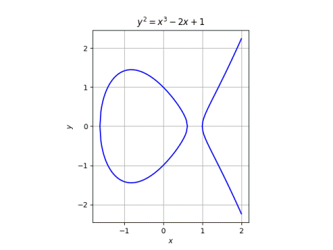
Elliptic curves are pure and applied, concrete and abstract, simple and complex.

Elliptic curves have been studied for many years by pure mathematicians with no intention to apply the results to anything outside math itself. And yet elliptic curves have become a critical part of applied cryptography.

Elliptic curves are very concrete. There are some subtleties in the definition—more on that in a moment—but they’re essentially the set of points satisfying a simple equation. And yet a lot of extremely abstract mathematics has been developed out of necessity to study these simple objects. And while the objects are in some sense simple, the questions that people naturally ask about them are far from simple.

y^2 = x^3 - 2x + 1

Preliminary definition

A preliminary definition of an elliptic curve is the set of points satisfying

y² = x³ + ax + b.

This is a theorem, not a definition, and it requires some qualifications. The values xya, and b come from some field, and that field is an important part of the definition of an elliptic curve. If that field is the real numbers, then all elliptic curves do have the form above, known as the Weierstrass form. For fields of characteristic 2 or 3, the Weierstrass form isn’t general enough. Also, we require that

4a³ + 27b² ≠ 0.

The other day I wrote about Curve1174, a particular elliptic curve used in cryptography. The points on this curve satisfy

x² + y² = 1 – 1174 x² y²

This equation does not specify an elliptic curve if we’re working over real numbers. But Curve1174 is defined over the integers modulo p = 2251 – 9. There it is an elliptic curve. It is equivalent to a curve in Weierstrass, though that’s not true when working over the reals. So whether an equation defines an elliptic curve depends on the field the constituents come from.

Not an ellipse, not a curve

An elliptic curve is not an ellipse, and it may not be a curve in the usual sense.

There is a connection between elliptic curves and ellipses, but it’s indirect. Elliptic curves are related to the integrals you would write down to find the length of a portion of an ellipse.

Working over the real numbers, an elliptic curve is a curve in the geometric sense. Working over a finite field, an elliptic curve is a finite set of points, not a continuum. Working over the complex numbers, an elliptic curve is a two-dimensional surface. The name “curve” is extended by analogy to elliptic curves over general fields.

Final definition

In this section we’ll give the full definition of an algebraic curve, though we’ll be deliberately vague about some of the details.

The definition of an elliptic curve is not in terms of equations of a particular form. It says an elliptic curve is a

  • smooth,
  • projective,
  • algebraic curve,
  • of genus one,
  • having a specified point O.

Working over real numbers, smoothness can be specified in terms of derivatives. But what does smoothness mean working over a finite field? You take the derivative equations from the real case and extend them by analogy to other fields. You can “differentiate” polynomials in settings where you can’t take limits by defining derivatives algebraically. (The condition 4a³ + 27b² ≠ 0 above is to guarantee smoothness.)

Informally, projective means we add “points at infinity” as necessary to make things more consistent. Formally, we’re not actually working with pairs of coordinates (xy) but equivalence classes of triples of coordinates (x, yz). You can usually think in terms of pairs of values, but the extra value is there when you need it to deal with points at infinity. More on that here.

An algebraic curve is the set of points satisfying a polynomial equation.

The genus of an algebraic curve is roughly the number of holes it has. Over the complex numbers, the genus of an algebraic curve really is the number of holes. As with so many ideas in algebra, a theorem from a familiar context is taken as a definition in a more general context.

The specified point O, often the point at infinity, is the location of the identity element for the group addition. In the post on Curve1174, we go into the addition in detail, and the zero point is (0, 1).

In elliptic curve cryptography, it’s necessary to specify another point, a base point, which is the generator for a subgroup. This post gives an example, specifying the base point on secp256k1, a curve used in the implementation of Bitcoin.

Microsoft replacing SHA-1

According to this article, Microsoft is patching Windows 7 and Windows Server 2008 to look for SHA-2 hash functions of updates. These older versions of Windows have been using SHA-1, while newer version are already using SHA-2.

This is a good move, but unnecessary. Here’s what I mean by that. The update was likely unnecessary for reasons I’ll explain below, but it was easy to do, and it increased consistency across Microsoft’s product line. It’s also good PR.

What are SHA-1 and SHA-2?

Let’s back up a bit. SHA-1 and SHA-2 are secure hash functions [1]. They take a file, in this case a Microsoft software update, and return a relatively small number, small relative to the original file size. In the case of SHA-1, the result is 160 bits (20 bytes).  They’re designed so that if a file is changed, the function value is nearly certain to change. That is, it’s extremely unlikely that a change to the file would not result in a change to the hash value.

The concern isn’t accidental changes. The probability of accidentally producing two files with the same hash function value is tiny as I show here.

The concern is a clever attacker who could modify the software update in such a way that the hash function remains unchanged, bypassing the hash as a security measure. That would be harder to do with SHA-2 than with SHA-1, hence Microsoft’s decision years ago to move to SHA-2 for new versions of the operating system, and its recent decision to make the change retroactive.

How hard is it to produce collisions?

By a collision we mean two files that hash to the same value. It’s obvious from the pigeon hole principle [2] that collisions are possible, but how hard are they to produce deliberately?

Google demonstrated two years ago that it could produce two PDF files with the same SHA-1 hash value. But doing so required over 6,500 years of CPU time running in parallel [3]. Also, Google started with a file designed to make collisions possible. According to their announcement,

We started by creating a PDF prefix specifically crafted to allow us to generate two documents with arbitrary distinct visual contents, but that would hash to the same SHA-1 digest.

It would be harder to start with a specified input, such as a software update file and generate a collision. It would be harder still to generate a collision that had some desired behavior.

According to this page, it’s known how to tamper with two files simultaneously so that they will have the same SHA-1 hash values. This is what Google did, at the cost of thousands of CPU years. But so far, nobody has been able to start with a given file and create another file with the same SHA-1 value. (Update: Now they have!)

As I said at the beginning, it made sense for Microsoft to decide to move from SHA-1 to SHA-2 because the cost of doing so was small. But the use of SHA-1 hash codes is probably not the biggest security risk in Windows 7.

More secure hash posts

[1] SHA-1 is a hash function, but SHA-2 is actually a family of hash functions: SHA-224, SHA-256, SHA-384, SHA-512, SHA-512/224, and SHA-512/256. All are believed to provide at least 112 bits of security, while SHA-1 provides less than 63.

The SHA-x functions output x bits. The SHA-x/y functions use x bits of internal state and output y bits. To be consistent with this naming convention, SHA-1 should be called SHA-160.

[2] The pigeon hole principle says that if you put more than n things into n boxes, one of the boxes has to have more than one thing. If you hash files of more than n bits to n-bit numbers, at least two files have to go to the same value.

[3] If you were to rent this much CPU time in the cloud at 5 cents per CPU hour, it would cost about $2,800,000. If the only obstacle were the cost of computing resources, someone might be willing to pay that to tamper with a Microsoft update. (Update: with a new algorithm announced in January 2020, the estimated cost has dropped $45,000.)

Hash function menagerie

Here’s an oversimplified survey of cryptographic hash functions: Everyone used to use MD5, now they use some variation on SHA.

There’s some truth to that. MD5 was very popular, and remains popular years after it was proven insecure. And now variations on SHA like SHA1 and SHA256 are commonly used. But there are a lot more cryptographic hash functions in common use.

Python support

If Python’s hashlib is a reliable guide, the most common hashing algorithms are

  • MD5
  • SHA1
  • SHA224
  • SHA256
  • SHA384
  • SHA512

because these are the six algorithms guaranteed to be supported on every platform, as listed in the output of the algorithms_guaranteed method in hashlib.

The algorithms_available methods in hashlib includes additional algorithms available in a particular installation. On the computer I’m using at the moment, it lists 18 hash algorithms in addition to those on the guaranteed list.

Mathematica support

Mathematica supports the hash functions on hashlib‘s guaranteed list, and a few more:

  • Adler32
  • CRC32
  • MD3
  • MD4
  • RIPEMD160
  • RIPEMD160SHA256
  • SHA256SHA256

The first two hashes, Adler32 and CRC32, were never intended to be secure. They were designed simply as error detection codes and weren’t designed to be tamper-resistant. As the names imply, MD3 and MD4 were predecessors to MD5.

The hash that Mathematica calls RIPEMD160SHA256 is SHA 256 followed by the RIPEMD160. The reason this combination gets a name of its own is because it is used in Bitcoin. Finally, SHA256SHA256 is simply SHA256 applied twice.

The long tail

The hash functions mentioned above are the most commonly used, but there are hundreds of others in common use. The hashcat password cracking tool lists 260 kinds of hash functions it can attack.

Some of these hash functions are fundamental algorithms, such as Whirlpool and variations of GOST. Some are combinations of primitive functions, such as salted or iterated variations. Many of them are vendor and product specific. For example, hashcat lists nine different hashing algorithms associated with various versions of Microsoft Office, six algorithms for Cisco products, five algorithms for SAP, etc.

It’s interesting to speculate on why there are so many custom hash functions: hashing technology progress, differing emphases on security and speed, not-invented-here syndrome, etc.

Security by variety

There’s something going on that isn’t exactly security-by-obscurity, i.e. relying on keeping your encryption algorithm a secret. The hashing algorithms for all the products mentioned above are well known, but there may be some small advantage to being a little bit off the beaten path.

People have built special hardware and software for attacking popular hashing algorithms, and doing something a little different could prevent this from working on your hash. Of course doing something a little different could also introduce a weakness you didn’t anticipate. Creating your own encryption algorithm is a bad idea unless you’re an expert, and often even if you are an expert. But making a new hash function by combining secure primitives is not as dangerous as creating your own encryption algorithm.

More hash function posts