Optimization, Dominoes, and Frankenstein

Robert Bosch has a new book coming out next week titled OPT ART: From Mathematical Optimization to Visual Design. This post will look at just one example from the book: creating images of Frankenstein’s monster [1] using dominoes.

Frankenstein made from 3 sets of double nine dominoes

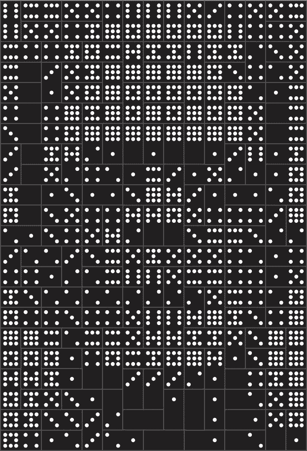
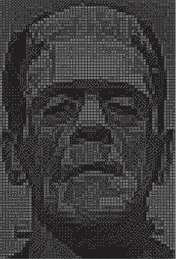
The book includes two images, a low-resolution image made from 3 sets of dominoes and a high resolution image made from 48 sets. These are double nine dominoes rather than the more common double six dominoes because the former allow a more symmetric arrangement of dots. There are 55 dominoes in a double nine set. (Explanation and generalization here.)

Image of Frankenstein's monster made from 48 sets of double nine dominoes

The images are created by solving a constrained optimization problem. You basically want to use dominoes whose brightness is proportional to the brightness of the corresponding section of a photograph. But you can only use the dominoes you have, and you have to use them all.

You would naturally want to use double nines for the brightest areas since they have the most white spots and double blanks for the darkest areas. But you only have three of each in the first image, forty eight of each in the second, and you have to make do with the rest of the available pieces. So you solve an optimization problem to do the best you can.

Each domino can be places horizontally or vertically, as long as they fit the overall shape of the image. In the first image, you can see the orientation of the pieces if you look closely. Here’s a little piece from the top let corner.

Domino orientation

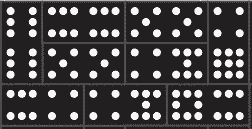
One double six is placed vertically in the top left. Next to it are another double six and a double five placed horizontally, etc.

There are additional constraints on the optimization problem related to contrast. You don’t just want to match the brightness of the photograph as well as you can, you also want to maintain contrast. For example, maybe a five-two domino would match the brightness of a couple adjacent squares in the photograph, but a seven-one would do a better job of making a distinction between contrasting regions of the image.

Bosch explains that the problem statement for the image using three sets of dominoes required 34,265 variables and 385 domino constraints. It was solved using 29,242 iterations of a simplex algorithm and required a little less than 2 seconds.

The optimization problem for the image created from 48 sets of dominoes required 572,660 variables and 5,335 constraints. The solution required 30,861 iterations of a simplex algorithm and just under one minute of computation.

Related posts

[1] In the Shelley’s novel Frankenstein, the doctor who creates the monster is Victor Frankenstein. The creature is commonly called Frankenstein, but strictly speaking that’s not his name. There’s a quote—I haven’t been able to track down its source—that says “Knowledge is knowing that Frankenstein wasn’t the monster. Wisdom is knowing that Frankenstein was the monster.” That is, the monster’s name wasn’t Frankenstein, but what Victor Frankenstein did was monstrous.

More on attacking combination locks

A couple weeks ago I wrote about how De Bruijn sequences can be used to attack locks where there is no “enter” key, i.e. the lock will open once the right symbols have been entered.

Here’s a variation on this theme: what about locks that let you press more than one button at a time? [1]

Lock that lets you push more than one button at a time

You could just treat this as if it were a keypad with more buttons. For example, suppose you can push either one or two buttons at a time on the lock pictured above. Then you could treat this as a lock with 15 buttons: the five actual buttons and 10 virtual buttons corresponding to the ten ways you could choose 2 buttons out of 5 to press at the same time.

Maybe a lock would let you press even more buttons at once. I don’t think I’ve ever used a combination that required more than two buttons at once, but in principle you could push up to five buttons at once in the photo above, for a total of 31 possible button combinations. And since 31 is prime, you could use the algorithm here to generate the corresponding De Bruijn sequence.

If you know how long the password is, you can try the De Bruijn sequence for passwords of that length. But what if you don’t know the length of the password a priori? You could try the De Bruijn sequence for passwords of length 1, then length 2, then length 3, etc. But is there a more efficient way?

If there are k button combinations and the password has length n, then the optimal solution is to start entering a De Bruijn sequence B(k, n) until the lock opens. If you know the password has length no more than 4, then you could try a B(k, 4) sequence, and if the password is actually shorter than 4, say length 3, you’ll still open it.

But what if you’ve tried a B(k, 4) sequence and it turns out the password has length 5? You could do better than starting over with a B(k, 5) sequence, because some of the substrings in that B(k, 5) sequence will have already been tried. But how could you do this systematically? If you don’t know the length of the password, how could you do better than trying B(k, 1), then B(k, 2), then B(k, 3) etc.?

Related posts

[1] For this post, I’m assuming the lock will open as soon as you enter the right sequence of buttons. For example, if the pass code is 345 and you enter 12345 the lock will open. I don’t know whether these locks work that way. Maybe you have to turn the handle, which would effectively act as an enter key. But maybe there’s a way to listen to the lock so that you’ll know when the combination has been entered, before you twist the handle.

Update: According to the first comment below, locks of the kind featured in the photo only allow each button to be used once. That puts severe limits on the number of possible combinations, and the approach outlined here would be unnecessary. However, the post brings up more general questions that could be useful in another setting.

Summing an array of floating point numbers

Adding up an array of numbers is simple: just loop over the array, adding each element to an accumulator.

Usually that’s good enough, but sometimes you need more precision, either because your application need a high-precision answer, or because your problem is poorly conditioned and you need a moderate-precision answer [1].

There are many algorithms for summing an array, which may be surprising if you haven’t thought about this before. This post will look at Kahan’s algorithm, one of the first non-obvious algorithms for summing a list of floating point numbers.

We will sum a list of numbers a couple ways using C’s float type, a 32-bit floating point number. Some might object that this is artificial. Does anyone use floats any more? Didn’t moving from float to double get rid of all our precision problems? No and no.

In fact, the use of 32-bit float types is on the rise. Moving data in an out of memory is now the bottleneck, not arithmetic operations per se, and float lets you pack more data into a giving volume of memory. Not only that, there is growing interest in floating point types even smaller than 32-bit floats. See the following posts for examples:

And while sometimes you need less precision than 32 bits, sometimes you need more precision than 64 bits. See, for example, this post.

Now for some code. Here is the obvious way to sum an array in C:

    float naive(float x[], int N) {
        float s = 0.0;
        for (int i = 0; i < N; i++) {
            s += x[i];
        }
        return s;
    }

Kahan’s algorithm is not much more complicated, but it looks a little mysterious and provides more accuracy.

    float kahan(float x[], int N) {
        float s = x[0];
        float c = 0.0;
        for (int i = 1; i < N; i++) {
            float y = x[i] - c;
            float t = s + y;
            c = (t - s) - y;
            s = t;
        }
        return s;
    }

Now to compare the accuracy of these two methods, we’ll use a third method that uses a 64-bit accumulator. We will assume its value is accurate to at least 32 bits and use it as our exact result.

    double dsum(float x[], int N) {
        double s = 0.0;
        for (int i = 0; i < N; i++) {
            s += x[i];
        }
        return s;
    }

For our test problem, we’ll use the reciprocals of the first 100,000 positive integers rounded to 32 bits as our input. This problem was taken from [2].

    #include <stdio.h>
    int main() {
        int N = 100000;
        float x[N];
        for (int i = 1; i <= N; i++)
            x[i-1] = 1.0/i;
  
        printf("%.15g\n", naive(x, N));
        printf("%.15g\n", kahan(x, N));  
        printf("%.15g\n", dsum(x, N));
    }

This produces the following output.

    12.0908508300781
    12.0901460647583
    12.0901461953972

The naive method is correct to 6 significant figures while Kahan’s method is correct to 9 significant figures. The error in the former is 5394 times larger. In this example, Kahan’s method is as accurate as possible using 32-bit numbers.

Note that in our example we were not exactly trying to find the Nth harmonic number, the sum of the reciprocals of the first N positive numbers. Instead, we were using these integer reciprocals rounded to 32 bits as our input. Think of them as just data. The data happened to be produced by computing reciprocals and rounding the result to 32-bit floating point accuracy.

But what if we did want to compute the 100,000th harmonic number? There are methods for computing harmonic numbers directly, as described here.

Related posts

[1] The condition number of a problem is basically a measure of how much floating point errors are multiplied in the process of computing a result. A well-conditioned problem has a small condition number, and a ill-conditioned problem has a large condition number. With ill-conditioned problems, you may have to use extra precision in your intermediate calculations to get a result that’s accurate to ordinary precision.

[2] Handbook of Floating-Point Arithmetic by Jen-Michel Muller et al.

Any number can start a factorial

Any positive number can be found at the beginning of a factorial. That is, for every positive integer n, there is an integer m such that the leading digits of m! are the digits of n.

There’s a tradition in math to use the current year when you need an arbitrary numbers; you’ll see this in competition problems and recreational math articles. So let’s demonstrate the opening statement with n = 2019. Then the smallest solution is m = 3177, i.e.

3177! = 2019…000

The factorial of 3177 is a number with 9749 digits, the first of which are 2019, and the last 793 of which are zeros.

The solution m = 3177 was only the first. The next solution is 6878, and there are infinitely more.

Not only does every number appear at the beginning of a factorial, it appears at the beginning of infinitely many factorials.

We can say even more. Persi Diaconis proved that factorials obey Benford’s law, and so we can say how often a number n appears at the beginning of a factorial.

If a sequence of numbers, like factorials, obeys Benford’s law, then the leading digit d in base b appears with probability

logb(1 + 1/d).

If we’re interested in 4-digit numbers like 2019, we can think of these as base 10,000 digits [1]. This means that the proportion factorials that begin with 2019 equals

log10000(1 + 1/2019)

or about 1 in every 18,600 factorials.

By the way, powers of 2 also obey Benford’s law, and so you can find any number at the beginning of a power of 2. For example,

22044 = 2019…

Related: Benford’s law blog posts

[1] As pointed out in the comments, this approach underestimates the frequency of factorials that start with 2019. It would count numbers of the form 2019 xxxx xxxx, but not numbers of the form 201 9xxx xxxx etc. The actual frequency would be 4x higher.

Arbitrary precision is not a panacea

Having access to arbitrary precision arithmetic does not necessarily make numerical calculation difficulties go away. You still need to know what you’re doing.

Before you extend precision, you have to know how far to extend it. If you don’t extend it enough, your answers won’t be accurate enough. If you extend it too far, you waste resources. Maybe you’re OK wasting resources, so you extend precision more than necessary. But how far is more than necessary?

As an example, consider the problem of finding values of n such that tan(n) > n discussed a couple days ago. After writing that post, someone pointed out that these values of n are one of the sequences on OEIS. One of the values on the OEIS site is

k = 1428599129020608582548671.

Let’s verify that tan(k) > k. We’ll use our old friend bc because it supports arbitrary precision. Our k is a 25-digit number, so lets tell bc we want to work with 30 decimal places to give ourselves a little room. (bc automatically gives you a little more room than you ask for, but we’ll ask for even more.)

bc doesn’t have a tangent function, but it does have s() for sine and c() for cosine, so we’ll compute tangent as sine over cosine.

    $ bc -l
    scale = 30
    k = 1428599129020608582548671
    s(k)/c(k) - k

We expect this to return a positive value, but instead it returns

-1428599362980017942210629.31…

So is OEIS wrong? Or is bc ignoring our scale value? It turns out neither is true.

You can’t directly compute the tangent of a large number. You use range reduction to reduce it to the problem of computing the tangent of a small angle where your algorithms will work. Since tangent has period π, we reduce k mod π by computing k − ⌊k/π⌋π. That is, we subtract off as many multiples of π as we can until we get a number between 0 and π. Going back to bc, we compute

    pi = 4*a(1)
    k/pi

This returns

    454737226160812402842656.500000507033221370444866152761

and so we compute the tangent of

    t = 0.500000507033221370444866152761*pi
      = 1.570797919686740002588270178941

Since t is slightly larger than π/2, the tangent will be negative. We can’t have tan(t) greater than k because tan(t) isn’t even greater than 0. So where did things break down?

The calculation of pi was accurate to 30 significant figures, and the calculation of k/pi was accurate to 30 significant figures, given our value of pi. So far has performed as promised.

The computed value of k/pi is correct to 29 significant figures, 23 before the decimal place and 6 after. So when we take the fractional part, we only have six significant figures, and that’s not enough. That’s where things go wrong. We get a value ⌊k/π⌋ that’s greater than 0.5 in the seventh decimal place while the exact value is less than 0.5 in the 25th decimal place. We needed 25 − 6 = 19 more significant figures.

This is the core difficulty with floating point calculation: subtracting nearly equal numbers loses precision. If two numbers agree to m decimal places, you can expect to lose m significant figures in the subtraction. The error in the subtraction will be small relative to the inputs, but not small relative to the result.

Notice that we computed k/pi to 29 significant figures, and given that output we computed the fractional part exactly. We accurately computed ⌊k/π⌋π, but lost precision when we computed we subtracted that value from k.

Our error in computing k − ⌊k/π⌋π was small relative to k, but not relative to the final result. Our k is on the order of 1025, and the error in our subtraction is on the order of 10−7, but the result is on the order of 1. There’s no bug in bc. It carried out every calculation to the advertised accuracy, but it didn’t have enough working precision to produce the result we needed.

Related posts