Exact sequences

A couple days ago, near the end of a post, I mentioned exact sequences. This term does not mean what you might reasonably think it means. It doesn’t mean exact in the sense of not being approximate.

It means that the stuff that comes out of one step is exactly the stuff that gets set to 0 in the next step. That is, the image of each function is exactly the kernel of the next function in the sequence [1].

Gradient and curl

For example, let f be gradient and let g be curl. Then the following sequence is exact

A \to^f B \to^g C

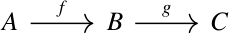
if A is the set of smooth functions from ℝ³ to ℝ, and B and C are set of smooth functions ℝ³ to ℝ³.

This says that the image of f, vector fields that are the gradient of something, is the kernel of g, vector fields with zero curl. In other lingo, gradient vector fields are irrotational, and all irrotational vector fields are the gradient of some potential function.

To show that

image f = kernel g

we have to show two things:

image f ⊂ kernel g

and

image f ⊃ kernel g

As is often the case, the former is easier than the latter. It’s a common homework problem [2] to show that the curl of a divergence is zero, i.e.

∇×(∇φ) = 0

It’s not so easy to show that for every vector field F with ∇×F = 0 there exists a potential φ such that F = ∇φ. It’s easier to show that the image of the first function part of the kernel of the next than to show that the kernel of the first is exactly the kernel of the next, because the latter requires proving the existence of something.

Short exact sequences

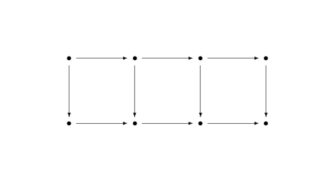
A short exact sequence is an exact sequence of the following form. (It’s called short because exact sequences are often longer.)

0 \to A \to^f B \to^g C \to 0

There’s no label on the arrow from 0 to A because there’s only one function from 0 to anywhere. There’s also no label on the arrow from C to 0 because there’s only one function that goes from anywhere to 0 [3].

The zero on the left implies that the function f is one-to-one (injective). It’s image is only one element, so the kernel of f is only one element.

Similarly the zero on the right end implies that the function g is onto (surjective). The kernel of the last arrow is everything in C, so the image of g has to be everything in C.

For example, let B be a group and suppose φ is a homomorphism from B to another group. Let A be the kernel of φ and let f be the inclusion map from the kernel into B. Let g be quotient map taking C = B/A. Then the so-called “first group homomorphism theorem” says that the sequence above is exact.

Div, grad, curl and all that

The title of this section is an homage to an excellent little book by H. M. Schey.

We said above that the curl of a gradient is zero, and that all vector fields with zero curl are gradients. It’s also true that the divergence of a curl is zero, and that a vector field is has zero divergence if it is the curl of something. That is, for a vector field F,

∇ · (∇ × F) = 0

and if ∇ · G = 0 for a vector field G then there exists a vector field F such that

∇×F = G.

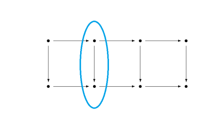
This means we can extend our example above to

0 \to A \to^{grad} B \to^{curl} C \to^{div} D \to 0

if we define A carefully.

The discussion in this section only justifies the labeled arrows. We need to justify the two unlabeled arrows on the ends.

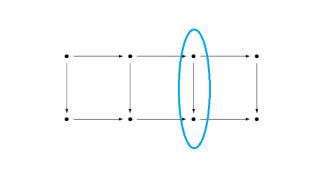
The zero on the left requires the gradient be one-to-one. But in general, the gradient is not one-to-one: functions that differ by a constant have the same gradient. But if we define A to be the set of integrable functions on ℝ³ then the gradient is one-to-one. Requiring the integral of a function over ℝ³ to exist means the functions must eventually approach zero in every direction.

The zero on the right requires every smooth function on ℝ³ to be the divergence of something. That’s easy. Given a function φ from ℝ³ to ℝ, let F be the vector field whose first component at (x, y, z) is the integral of φ from the origin to (x, 0, 0) and whose second and third components are 0. Then the divergence of F equals φ.

Long(er) exact sequences

The exact sequence in the previous section is longer than a short exact sequence, and longer exact sequences come up in practice. An exact sequence could be infinite in one or both directions. For example, the Mayer–Vietoris sequence, a foundational tool in homology, is infinite on its left and terminates in 0 on its right end.

Related posts

[1] The term “zero” is overloaded here. It could be the integer 0, or the origin of a vector space, or the kernel of a group, etc.

Everything here generalizes to objects and morphisms in a category, in which case the objects are not necessarily sets, and the morphisms are not necessarily functions. Then we don’t talk about images and kernels but about morphisms being monomorphisms and epimorphisms.

[2] There is a lot of foreshadowing in textbooks. It’s common for an author to include exercises and examples that are important later. This is often intentional, sort of an Easter egg. But sometimes the author is unconsciously pulling from experience.

[3] This observation is turned into a definition in category theory: a zero object is defined as one that is initial and final. That is, there is only one morphism from it to any other object, and only one morphism from any object to it.

Data swamps

swamp

I recently heard the term data swamp, a humorous take on data lakes. I thought about data swamps yesterday when I hiked past the literal swamp in the photo above.

Swamps are a better metaphor than lakes for heterogeneous data collections because a lake is a homogeneous body of water. What makes a swamp a swamp is its heterogeneity.

The term “data lake” may bring up images of clear water, maybe an alpine lake like Lake Tahoe straddling California and Nevada. “Data swamp” makes me think of Louisiana’s Atchafalaya Basin, which is probably a more appropriate image for most data lakes.

Related posts

Numerical footnote

Yesterday’s post said that that you could construct a chain of linear relationships between the hypergeometric function

F(a, b; c; z)

and

F(a+i, b+j; c+k; z)

for integers i, j, and k. Toward the end of the post I said that this could be used to speed up programs by computing function values from previous values rather than from scratch. This is true, but you need to check whether there are numerical issues.

You have to be careful when using recurrence relations numerically. It’s common for a recurrence to be numerically stable in one direction but unstable in the opposite direction. I wrote about this here and gave examples.

The stability problems for recurrence relations are the discrete analog of the more familiar problem of sensitive dependence on initial conditions for differential equations described here.


Four, five, and nine lemmas

This post is similar in spirit to the previous post: reducing mathematical theorems to moves in a board game by looking at things from a ridiculously high level.

The theorems we’ll be looking at are known as the four lemma, the five lemma, and the nine lemma. The nine lemma is also known as the 3×3 lemma.

All the lemmas start with a commutative diagram. A diagram is commutative if any two ways of getting from one place to another are equal. If the arrows represent functions, then the diagram implies certain compositions of functions are equal.

Given hypotheses about most of the arrows in a diagram, the theorems conclude something about the rest of the arrows. This general category of theorems is known as diagram chasing. The proofs are tedious but shallow. If a theorem in topology, for example, were formulated as a diagram chase, someone with no intuition for topology could prove the theorem by applying the rules of a simple game.

The meaning of the dots and arrows isn’t important for this post, but you could think of the dots in the diagram as groups and the arrows as homomorphisms between groups. More generally you could think of the dots as objects in an Abelian category and the arrows as morphisms between objects.

The four lemma

The four lemma starts with a commutative diagram of the following shape.

It’s called the four lemma because there are four dots across each row.

There are two versions of the four lemma. Both make assumptions about the rows and three out of the four columns and conclude something about the fourth column.

In the first part of the lemma, we have hypotheses about the two rows, and hypotheses about the first, third, and fourth vertical arrows. The conclusion is something about the second vertical arrow.

The second part of the lemma is very similar, but has hypotheses about the first, second, and fourth vertical arrows and concludes something about the third arrow.

Five lemma

The five lemma starts with a commutative diagram with five objects across the top and bottom rows.

Given assumptions about every arrow except the vertical arrow in the middle, the theorem concludes something about the middle arrow.

Nine lemma

The nine lemma, a.k.a. the 3×3 lemma, starts with a commutative diagram of the following shape.

It’s called the nine lemma because the attention is focused on the nine dots, the 3×3 grid of dots in the middle. All the objects around the perimeter, those outside the 3×3 grid, are 0.

There are three parts to the nine lemma. Each has hypotheses about all the columns and two of the rows, and concludes something about the row that was left out. So, for example, one part of the theorem has hypotheses about the three columns and the first two rows and concludes something about the last row.

Missing details

Here I zoom in from 100,000 feet to 10,000 feet, giving some of the missing details but not all. For full details, you could look up the theorems on Wikipedia or on nLab.

As promised at the beginning, this was a ridiculously high-level view of these theorems. The purpose was to point out the core of each theorem and making it possible to compare the three theorems at the highest level.

When I said a theorem makes a hypothesis about a row or a column, the hypothesis is that the row forms an exact sequence. The conclusions in the nine lemma are that a row is an exact sequence.

When I alluded to hypotheses about vertical arrows, these hypotheses are essentially saying that a function is one-to-one (injective), onto (surjective), or one-to-one and onto (bijective). More precisely, they are assumptions that a morphism is mono, epi, or iso. More on this terminology here. The conclusion of the four lemma is that an arrow is either epi or mono. The conclusion of the five lemma is that an arrow is iso.

Related posts

T test with unequal variances

The test statistic in the t-test does not exactly follow a Student t distribution except under ideal conditions.

If you’re comparing data from two normally distributed populations to see whether they have the same mean, the test statistic for the two-sample t-test does not have a t distribution unless the two populations have equal variance.

Robustness

Maybe this isn’t a problem. Your data didn’t exactly come from a normal distribution, so maybe it doesn’t matter that the test statistic doesn’t exactly have a t distribution. It’s a matter of robustness.

I’ve written before about the robustness of the t-test to violations of the normality assumption. In that post I assumed two populations have the same variance, but not a normal distribution. The conclusion was that departures from the normal distribution don’t matter so much, but departures from symmetry do.

For this post we’ll keep the normality assumption but have unequal variances. We know that the distribution of the test statistic is approximately, but not exactly, a t distribution. But what distribution does it have? I’ve seen it called “not pleasant” [1] but I haven’t seen a plot of it, so I’m curious.

Details

Suppose we have n samples from a random variable X and m samples from a random variable Y, and that the sample variances for the two samples are sX and sY respectively. Our test statistic for equality of the two means is

T = \frac{\bar{X} - \bar{Y}}{\sqrt{\dfrac{s_x^2}{n} + \dfrac{s_Y^2}{m}}}

Sattertwhaite’s approximation for the distribution on T is a Student t distribution with degrees of freedom equal to

\hat{\nu} = \frac{\left(\dfrac{s_X^2}{n} + \dfrac{s_Y^2}{m} \right )^2 }{\dfrac{s_X^4}{n^2(n-1)} + \dfrac{s_Y^4}{n^2(n-1)}}

This is known as the Welch-Satterthrwaite equation.

There are numerous minor variations on the two-sample t-test, and the one using degrees of freedom in the Welch-Satterthrwaite equation is known as Welch’s t-test.

Simulation

For simulation I let X be a normal random variable with mean 100 and standard deviation 1, and Y be a normal random variable with mean 100 and standard deviation 50. I drew 15 samples from X and 12 from Y and computed the statistic T. I did this 10,000 times and plotted a histogram of the values of T. The result has very nearly a t distribution.

At least in this example, any deviance from the t distribution is minor. Welch’s t-test is said to be robust to differences in variance, and this is an example of it living up to its reputation.

Related posts

[1] Casella and Berger, Statistical Inference.

3D Go with identities

Let’s play a game that’s something like Go in three dimensions. Our game is played on the lattice of points in 3D that have integer coordinates. Someone places stones on two lattice points, and your job is to create a path connecting the two stones by adding stones to neighboring locations.

Game cube

We don’t really have a game “board” since we’re working in three dimensions. We have a game scaffold or game cube. And we can’t just put our stones down. We have to imagine the stones has having hooks that we can use to hang them where pieces of scaffolding come together.

Basic moves

Now for the rules. Our game is based on identities for a function with depending on three parameters: a, b, and c. A location in our game cube is a point with integer coordinates (i, j, k) corresponding to function parameters

(a+i, b+j, c+k).

If there is a stone at (i, j, k) then we are allowed to place stones at neighboring locations if there is a function identity corresponding to these points. The function identities are the “contiguous relations” for hypergeometric functions. You don’t need to know anything about hypergeometric functions to play this game. We’re going to leave out a lot of detail.

Our rule book for identities will be Handbook of Mathematical Function by Abramowitz and Stegun, widely known as A&S. You can find a copy online here.

For example, equation 15.2.10 from A&S relates

F(a, b; c; z)

to

F(a-1, b; c; z)

and

F(a+1, b; c; z).

So if we have a stone at (i, j, k) we can add stones at (i-1, j, k) and (i+1, j, k). Or we could add stones at (i+1, j, k) and (i+2, j, k). You can turn one stone into a row of three stones along the first axis overlapping the original stone.

Equation 15.2.11 lets you do something analogous for incrementing the 2nd coordinate, and Equation 15.2.12 lets you increment the 3rd coordinate. So you could replace a stone with a row of three stones along the second or third axes as well.

This shows that it is always possible to create a path between two lattice points. If you can hop between stones a distance 1 apart, you can create a path that will let you hop between any two points.

Advanced moves

There are other possible steps. For example, equation 15.2.25 has the form

F(a, b; c; z) + … F(a, b-1; c; z)  + … F(a, b; c+1; z) = 0

I’ve left out the coefficients above, denoting them by ellipses. (More on that below.) This identity says you don’t just have to place stones parallel to an axis. For example, you can add a stone one step south and another one step vertically in the same move.

The previous section showed that it’s always possible to create a path between two lattice points. This section implies the finding the shortest path between two points might be a little more interesting.

Applications

There are practical applications to the game described in this post. One reason hypergeometric functions are so useful is that they satisfy a huge number of identities. There are libraries of hypergeometric identities, and there are still new identities to discover and new patterns to discover for organizing the identities.

The moves in the game above can be used to speed up software. Hypergeometric functions are expensive to evaluate, and so it saves time to compute a new function in terms of previously computed functions rather than having to compute it from scratch.

I used this trick to speed up clinical trial simulations. Consecutive steps in the simulation required evaluating contiguous hypergeometric functions, so I could compute one or two expensive functions at the beginning of the simulation and bootstrap them to get the rest of the values I needed.

Coefficients

I’d like to close by saying something about the coefficients in these identities. The coefficients are complicated and don’t have obvious patterns, and so they distract from the underlying structure discussed here. You could stare at a list of identities for a while before realizing that apart from the coefficients the underlying relationships are simple.

All the coefficients in the identities cited above are polynomials in the variables a, b, c, and z. All have degree at most 2, and so they can be computed quickly.

The identities discussed here are often called linear relations. The relations are linear in the hypergeometric functions, but the coefficients are not linear.

Related posts