Runge-Kutta order versus stages

Posted on 1 August 2026 by John

The textbook version of the Runge-Kutta method for solving differential equations has 4 stages and has 4th order error. For lower order versions of RK the number of stages s also matches the order of the error p. But in order to achieve error on the order of p ≥ 5, you need more than p stages. This is known as the Butcher barrier.

Before going any further, let’s back up and say what we mean by stages and by order.

Stages

The number of stages in an RK method to solve the equation

y' = f(t, y)

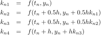
is the number of evaluations of the function f on the right-hand side. For example, the textbook RK4 method estimates the solution at each step by

$y_{n+1} = y_n + \frac{h}{6}\left( k_{n1} + 2k_{n2} + 2k_{n3} + k_{n4}\right)$

where

$k_{n1} &=& f(t_n, y_n) \\ k_{n2} &=& f(t_n + 0.5h, y_n + 0.5hk_{n1}) \\ k_{n3} &=& f(t_n + 0.5h, y_n + 0.5hk_{n2}) \\ k_{n4} &=& f(t_n + h, y_n + hk_{n3}) \\$

which requires four stages, i.e. four evaluations of f.

Order

A differential equation solver is said to have order p if the local error, the error after one step of size h, is O(h^{p + 1}). Then after solving an ODE over a period of time T with N = T/h steps, the global error is O(h^p). So, for example, if p = 4, you would expect that cutting your step size h in half would cut your error at T by a factor of 16.

More stages than the order

John C. Butcher proved that an explicit RK method of order p requires s stages where s > p if p > 4.

An important example is the Dormand-Prince method. It is a version of RK that has order 5 and 7 stages. The clever thing about this method is that you can make a 4th order solver out of a subset of its function evaluations.

That means that after you’ve evaluated one step of the 5th order method, you can also evaluate a 4th order method essentially for free. And by comparing them, you can get a sense of the error. If the solutions given by the two methods are substantially different, you have probably taken too big a step and need to back up. If the two solutions essentially agree, you’re probably good to take the next step.

For an explicit RK method to have order 5, 6, or 7 you need at least 6, 7, or 9 stages respectively.

Solving the RK4 design equations

Posted on 31 July 2026 by John

I was digging into the Runge-Kutta method for solving differential equations and a line from [1] piqued my curiosity.

These calculations, which are not reproduced in Kutta’s paper (they are however in Huen (1900)), are very tedious.

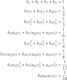
The calculations are a set of eight constraints that the parameters of a fourth-order Runge-Kutta method must satisfy. I wondered how well Mathematica might have done at assisting Mr. Huen in his “very tedious” calculations if it had been available in 1900.

I go into Runge-Kutta methods in this post. Here I’d like to concentrate on a step in the design of the methods, namely solving the set of equations alluded in the quote above.

$\begin{align*} b_1 + b_2 + b_3 + b_4 &= 1 \\ b_2 c_2 + b_3 c_3 + b_4 c_4 &= \frac{1}{2} \\ b_2 c_2^2 + b_3 c_3^2 + b_4 c_4^2 &= \frac{1}{3} \\ b_3 a_{32} c_2 + b_4(a_{42} c_2 + a_{43} c_3) &= \frac{1}{6} \\ b_2 c_2^3 + b_3 c_3^3 + b_4 c_4^3 &= \frac{1}{4} \\ b_3 c_3 a_{32} c_2 + b_4 c_4(a_{42} c_2 + a_{43} c_3) &= \frac{1}{8} \\ b_3 a_{32} c_2^2 + b_4(a_{42} c_2^2 + a_{43} c_3^2) &= \frac{1}{12} \\ b_4 a_{43} a_{32} c_2 &= \frac{1}{24} \end{align*}$

The first thing to note is that there are 10 variables and only 8 equations, and so the solution is not fully determined. What we think of as the fourth order Runge-Kutta method is in fact a fourth order Runge-Kutta method.

One could argue that we should have b₂ = b₃ and c₂ = c₃. With these additional equations, the system of equations has a unique solution, and Mathematica finds it easily.

eqs = {
    b1 + b2 + b3 + b4 == 1,
    b2*c2 + b3*c3 + b4*c4 == 1/2,
    b2*c2^2 + b3*c3^2 + b4*c4^2 == 1/3,
    b3*a32*c2 + b4*(a42*c2 + a43*c3) == 1/6,
    b2*c2^3 + b3*c3^3 + b4*c4^3 == 1/4,
    b3*c3*a32*c2 + b4*c4*(a42*c2 + a43*c3) == 1/8,
    b3*a32*c2^2 + b4*(a42*c2^2 + a43*c3^2) == 1/12,
    b4*a43*a32*c2 == 1/24,
    b2 == b3,
    c2 == c3
};

vars = {b1, b2, b3, b4, c2, c3, c4, a32, a42, a43};

solution = Solve[eqs, vars]

This returns the parameters used for the version of Runge-Kutta presented in every textbook.

If you keep the requirement b₂ = b₃ but substitute the requirement 2c₂ = c₃ for c‘s Mathematica will return the coefficients for the so-called Runge-Kutta 3/8 rule. This method has some slight advantages by some criteria.

In 1951 Gill [2] discovered a fourth order Runge-Kutta rule optimized for running in extremely constrained computer hardware. It’s a strange method, with irrational parameters, but one that was a very clever response to the limitations of its time.

Update: See this post for a discussion of the parameters and constraints for higher-ordered RK methods.

[1] Hairer, Nørsett, and Wanner. Solving Ordinary Differential Equations I: Nonstiff Problems. Springer-Verlag 1987.

[2] A. Gill. A process for the step-by-step integration of differential equations in an automatic digital computing machine. Proc. Cambridge Philos. Soc., vol 27, pp 95–108.

Inverse factorial improved

Posted on 28 July 2026 by John

A couple years ago I wrote about how to compute the inverse of factorial. I used that code in writing the previous post because the post required solving the equation

⌊log₂(n!)⌋ ≥ b

given b. That is, given a number of bits b, find the smallest value of n such that n! ≥ 2^b.

What the code got right

Looking back on the code in that post, there are a few changes I’d like to make. But first of all, I’d like to point out something the post does right: instead of trying to solve

Γ(y) = x

it solves

log Γ(y) = log x.

That’s why the argument to inverse_log_gamma is logarg. That makes the code useful for values of x that would far exceed the maximum floating point value, such as in the calculations for the previous post.

What I’d change

Rounding

The function inverse_factorial from the old post solves finds the closest integer solution. It would be better for it to return the solution without rounding and then let the user round result if they want to. In my calculations in the previous post, I wanted to take the floor, not round.

Newton’s method

The code in the previous post uses the bisection method. This method is very safe, and fast enough for my purposes, but it could be made faster. Newton’s method is faster, but it can be ill-behaved if you don’t start close enough to the solution.

It’s safe to use Newton’s method to invert log Γ for two reasons. First, you can get a good starting point based on Stirling’s approximation. Second, and more importantly, log Γ is convex. Newton’s method will converge from any starting point when applied to a convex function. A little caution is necessary because log Γ is not convex everywhere, but it is convex on the positive real axis.

Another difficulty with Newton’s method is that you need to supply the derivative of the function whose root you’re trying to find. But this isn’t an issue here because the derivative of log Γ is the digamma function, which is implemented in SciPy.

Tolerance

Finally, the previous code used the default tolerance for deciding when to stop refining the solution. The revised method lets the user specify tolerance. It provides a default value, but that default is visible in the function call, not hidden down in SciPy.

Revised code

Here’s the revised code.

from scipy.special import gammaln, digamma
from scipy.optimize import newton

def inverse_log_gamma(logarg, tol=1e-12):
    assert(logarg > 0)    
    x0 = logarg / log(logarg + 1) + 1 if logarg > 1 else 2.0
    def f(z): return gammaln(z) - logarg
    return newton(f, x0, fprime=digamma, tol=tol)

def inverse_factorial(logarg):
    g = inverse_log_gamma(logarg)
    return g - 1

Cryptographic Keys and Decks of Cards

Posted on 28 July 2026 by John

The previous post looked at the idea of storing a cryptographic key in the order of a deck of cards. A deck of 52 cards can store 225 bits of data because

⌊log₂(52!)⌋ = 225.

Here ⌊x⌋ is x rounded down to the nearest integer.

If we want to store bigger keys, we’re going to need a bigger deck of cards.

Bitcoin

A Bitcoin key has 256 bits, which would require a deck of 58 cards. There is a card game called Zwicker that uses a deck of 58 cards, the usual 52 cards plus six jokers. So you could store a Bitcoin key in the permutation of a Zwicker deck.

You could also use a deck of 52 cards, plus 2 jokers, if you also consider orientation. 30 cards are rotationally symmetric, 22 are not, and neither are jokers. So, including two asymmetric jokers, you could add 24 additional bits. Permutations of a 54 card deck can encode 237 bits, and with 24 orientation bits, this is a total of 261 bits.

RSA

RSA key sizes vary, but 2048 and 3072 are common. A 2048-bit key would require a deck of 301 cards. Casinos often use a shoe of 312 cards, combining six decks of 52 cards, to deal Baccarat or Blackjack. However, casinos combine identical decks. If you were to combine six unique decks, you could store a 2048-bit key.

Storing a 3072-bit key would require a deck of 422 cards. You could make a deck of 432 cards by combining 8 distinguishable packs of 54 cards (52 + 2 jokers).

ML-KEM

ML-KEM is a proposed quantum-resistant replacement for RSA. As with RSA, key sizes for ML-KEM vary, the smallest being ML-KEM-512 with a key size of 1632 bytes, which equals 13056 bits. This would require a deck of 1442 cards. You could combine 28 distinct packs of 52 cards, but that’s unwieldy.

This illustrates one of the difficult trade-offs with post-quantum cryptography: key sizes are much bigger. If you wanted to create a deck of 1442 cards, you’d probably want to make your “cards” something other than standard playing cards. You’d want to use permutations of something else.

Verification

The following Python code verifies the calculations above.

from math import log2, factorial, floor

def capacity(cards):
    return floor(log2(factorial(cards)))

def verify(bits, cards):
    return capacity(cards) >= bits and capacity(cards-1) < bits

print(verify(237, 54))
print(verify(256, 58))
print(verify(2048, 301))
print(verify(3072, 422))
print(verify(1632*8, 1442))

For more on how I came up with the deck sizes, see the next post on computing the inverse factorial.

Counting permutations with roots

Posted on 27 July 2026 by John

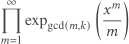
My post from yesterday on permutation roots ends with a Mathematica code for finding the probability that a permutation of n elements has a kth root. This is done by finding the coefficient of xⁿ in the generating function

$\prod_{m=1}^\infty \exp_{\text{gcd}(m, k)} \left\frac{x^m}{m}\right)$

I wanted to say more about this, and look at implementing the same code in SymPy. I was curious how well SymPy would do because I’ve noticed that LLMs often generate SymPy code since it’s an open source CAS.

Wilf [1] describes the infinite product above as the exponential generating function (egf) of f(n, k), the number of permutations of n objects that have a kth root. Since egfs have a n! term in the denominator, this is also the ordinary generating function (ogf) of the probability that a randomly chosen permutation on n objects has a kth root.

My first attempt at using Mathematica to probe the generating function was

expq[x_, q_] := MittagLefflerE[q, x^q]	 
p[n_, k_] :=  SeriesCoefficient[	 
    Product[expq[x^m/m, GCD[m, k]], {m, 1, Infinity}], {x, 0, n}]

This hung forever when I tried to use it on a small example. I realized, but apparently Mathematica did not, that Infinity could be replaced by n since terms higher than n do not contribute to the coefficient of xⁿ. With that change, the code ran quickly.

This morning I tried converting the Mathematica code to Sympy; Claude did this in one shot. I also reproduced the table of f(n, k) values on page 150 of [1] to test the code. Since Wilf tabulated f(n, k), not f(n, k)/n!, I multiplied the results by n!.

Here is the output:

k = 2 [1, 1, 3, 12, 60, 270, 1890, 14280, 128520, 1096200]
k = 3 [1, 2, 4, 16, 80, 400, 2800, 22400, 181440, 1814400]
k = 4 [1, 1, 3, 12, 60, 270, 1890, 13020, 117180, 1039500]
k = 5 [1, 2, 6, 24, 96, 576, 4032, 32256, 290304, 2612736]
k = 6 [1, 1, 1, 4, 40, 190, 1330, 8680, 52920, 340200]
k = 7 [1, 2, 6, 24, 120, 720, 4320, 34560, 311040, 3110400]

and here is the SymPy code. I edited the main but the rest is verbatim from Claude.

from sympy import symbols, gcd, factorial, Rational, S

x = symbols('x')

def expq_coeffs(m, q, n):
    """
    Truncated (degree <= n) series coefficients of
        expq(x**m/m, q) = MittagLefflerE(q, (x**m/m)**q)
    Since q is a positive integer:
        E_q(y^q) = sum_j y^(q*j) / (q*j)!
    with y = x**m/m, so the term of degree m*q*j has coefficient
        1 / ( m**(q*j) * (q*j)! ).
    Returns a list c[0..n] of coefficients.
    """
    c = [S.Zero] * (n + 1)
    j = 0
    while m * q * j <= n:
        deg = m * q * j
        c[deg] += Rational(1, m**(q * j) * factorial(q * j))
        j += 1
    return c

def poly_mult_trunc(a, b, n):
    """Multiply two series (lists of coeffs, index = degree) truncated to degree n."""
    c = [S.Zero] * (n + 1)
    for i, ai in enumerate(a):
        if ai == 0:
            continue
        max_j = n - i
        for j2 in range(max_j + 1):
            bj = b[j2]
            if bj != 0:
                c[i + j2] += ai * bj
    return c

def p(n, k):
    """
    SymPy equivalent of:
        expq[x_, q_] := MittagLefflerE[q, x^q]
        p[n_, k_] := SeriesCoefficient[
            Product[expq[x^m/m, GCD[m, k]], {m, 1, n}], {x, 0, n}]
    """
    result = [S.Zero] * (n + 1)
    result[0] = S.One
    for m in range(1, n + 1):
        q = gcd(m, k)
        factor = expq_coeffs(m, q, n)
        result = poly_mult_trunc(result, factor, n)
    return result[n]

# example
if __name__ == "__main__":
    for k in range(2, 8):
        print("k =", k, [factorial(n)*p(n, k) for n in range(1,11)])

[1] Herbert Wilf. Generatingfunctionology. Available online here.

Printing floating point numbers in binary

Posted on 27 July 2026 by John

It’s well known that you can convert the base 16 (hex) representation of an integer to the base 2 (binary) representation by simply converting each digit from hex to binary. For example,

CAFE_hex = 1100 1010 1111 1110_two

I imagine it’s less well known that you can do the same thing with floating point numbers.

I wanted to find the binary representation of a floating point number using Python, and discovered that it has no function to do this. However, there is a method on floats to show a hex representation. For example, here’s the hex representation of π.

>>> import math
>>> (math.pi).hex()
'0x1.921fb54442d18p+1'

Curiously, the p+k part at the end is an exponent of 2, not an exponent of 16. So after we convert 1.921fb54442d18 to binary, we’ll need to multiply by 2, i.e. move the fractional point one space to the right.

So first we convert 1.921fb54442d18_hex to binary by converting 1, 9, 2, etc. each to binary.

1.1001 0010 0001 1111 1011 0101 0100 0100 0100 0010 1101 0001 1000_two

Then after shifting the fraction point to account for the p+1 part we have

π = 11.001001000011111101101010100010001000010110100011000_two

You could use Python’s bin() function to convert the fractional part, interpreted as an integer, to hex, though you may need to pad with 0 bits. For example,

>>> (1.03).hex()
'0x1.07ae147ae147bp+0

>>> bin(0x7ae147ae147)
'0b1111010111000010100011110101110000101000111'

The binary representation of 1.03_ten is

1.000001111010111000010100011110101110000101000111_two

We added a total of five zero bits, four for the 0 after the fractional point and one for converting 7 to 0111_two.

exp_q

Posted on 26 July 2026 by John

The function exp_q(x) is defined by taking the power series for exp(x) and keeping only the terms whose index is a multiple of q. For example, exp₂(x) keeps only the even-numbered terms in the exponential power series and so equals cosh(x).

$\exp_2(x) = 1 + \frac{x^2}{2!} + \frac{x^4}{4!} + \frac{x^6}{6!} + \cdots = \cosh(x)$

In general,

$\exp_q(x) = \sum_{n=0}^\infty [q \mid n] \frac{x^n}{n!} = \sum_{n=0}^\infty \frac{x^{nq}}{(nq)!}$

The first sum uses Iverson’s bracket notation: a Boolean expression in brackets denotes the function that returns 1 when the expression is true and zero when it is false. Here the bracket equals 1 when q divides n and is zero otherwise.

Closed forms

Let ω = exp(2πi / q). Then

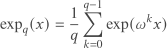
$\exp_q(x) = \frac{1}{q}\sum_{k=0}^{q-1} \exp(\omega^k x)$

This lets us find closed-form expressions for exp_q(x). For example, when q = 4, ω = i and

$\exp_4(x) = \frac{1}{2}\left( \cosh(x) + \cos(x) \right)$

Here’s a proof of the identity above:

$\begin{align*} \frac{1}{q} \sum_{k=0}^{q-1} \exp(\omega^k x) &= \frac{1}{q} \sum_{k=0}^{q-1} \sum_{n=0}^\infty \frac{\omega^{kn}x^n}{n!} \\ &= \sum_{n=0}^\infty \left( \frac{1}{q} \sum_{k=0}^{q-1} \omega^{kn}\right) \frac{x^n}{n!} \\ &= \sum_{n=0}^\infty [q \mid n] \frac{x^n}{n!} \\ &= \exp_q(x) \end{align*}$

In the proof we used the identity

$\frac{1}{q} \sum_{k=0}^{q-1} \omega^{kn} = [q \mid n]$

which is important in deriving the properties of the discrete Fourier transform.

Differential equations

The first time I saw the function exp_q(x) was in differential equations, though I didn’t know at the time the function had a name.

When a course in differential equations gets to power series solutions, a common example or homework problem is to solve

$y^{(k)}(x) = y(x)$

for k = 3 or 4, i.e. to find a function that equals its third or fourth derivative.

If the initial conditions are

and

$y^\prime(0) = y^{\prime\prime}(0) = \cdots = y^{(k-1)}(0) = 0$

the unique solution to

$y^{(k)}(x) = y(x)$

is y(x) = exp_k(x).

Mathematica and Mittag-Leffler

Mathematica does not have a built-in function implementing exp_q(x), but it does have an implementation of the Mittag-Leffler function, and so thanks to a relation between this function and exp_q(x) you can implement the latter as

expq[x_, q_] := MittagLefflerE[q, x^q]

Combinatorics

The first time I saw the notation exp_q(x) was in combinatorics. I had intended to include an application from that book here, but I make that the topic for the next post.

Excel column numbering

Posted on 25 July 2026 by John

I was working with a wide spreadsheet from a client the other day and I had to convert between Excel column labels and column numbers. I had never paid attention to how Excel labels columns and implicitly thought it was base 26 using letters rather than digits. But then I realized that’s not right.

Excel labels columns A through Z, then AA through AZ, then BA through BZ, etc. If this is base 26, then does A correspond to 0? That could work for A through Z, but then what about AA? Then you’d have to say the first A corresponds to 26 but the second A corresponds to 0.

Does Z correspond to 0? If so then the column numbers would be 1 through 25, followed by 0, then 27. And it would mean that columns ZA through ZZ are the same as A through Z.

In fact nothing in Excel column labeling corresponds to 0. The labels cannot be interpreted as a positional number system.

There’s a name for this kind of number system: bijective base 26. The concept extends generally to bijective base b for any positive integer b. The idea is ancient, but the name was coined recently. It has also been called k-adic numbering. For most of history it didn’t have a name.

The motivation behind the name bijective base b is that there is a bijection (a one-to-one correspondence) between these symbols and positive integers; there’s no possibility of leading zeros that would keep the mapping from being a bijection, unlike say 7 and 07 representing the same number.

Excel limits

Before 2007, an Excel file could have a maximum of 2⁸ = 256 columns, and so the largest column label was IV.

Then in 2007 the column limit was increased to 2¹⁴ = 16,384 and the largest column label is XFD.

Conversion code

Converting from column labels to integers is easy; going the other way is a little more complicated.

letter_to_ordinal = lambda c: ord(c) - ord('A') + 1
ordinal_to_letter = lambda n: chr(ord('A') + n - 1)

def label_to_num(label):
    label = label.upper()
    n = 0
    for c in label:
        n = n*26 + letter_to_ordinal(c)
    return n

def num_to_label(n):
    letters = []
    while n > 0:
        n, remainder = divmod(n - 1, 26)
        letters.append(ordinal_to_letter(remainder + 1))
    return ''.join(reversed(letters))

Here’s an online calculator based on the code above.

Tests

The following code verifies the assertions above about the maximum number of Excel columns over time.

assert(num_to_label(256) == "IV")
assert(label_to_num("IV") == 256)

assert(num_to_label(2**14) == "XFD")
assert(label_to_num("XFD") == 2**14)

The conversion routines are not limited to actual Excel labels but work for arbitrarily large integers and bijective base 26 representations. For example, the following code shows that the bijective base 26 representation of Avogadro’s number is MUAEKAUDYDXEWOSDD.

avogadro = 602_214_076_000_000_000_000_000
assert(label_to_num(num_to_label(avogadro)) == avogadro)
print(num_to_label(avogadro))

An almost periodic function

Posted on 23 July 2026 by John

This post takes a more abstract view of the previous post. That post looked at the concrete question of whether a number ever has the same sine in radians as in degrees. The relation between radians and degrees is irrelevant except that π/180 is an irrational number.

Suppose α and β are two positive numbers such that α/β is irrational. In the previous post, α = 1 and β = π/180. Then the function

f(x) = sin(αx) − sin(βx)

is almost periodic: it is not periodic, but it comes close to being periodic, as close as you’d like provided you’re willing to look over a sufficiently long range of x‘s.

The identity

sin(αx) − sin(βx) = 2 cos((α + β)x/2) sin((α − β)x/2)

shows that f(x) is the product of two periodic functions but is not periodic itself. The periods of the cosine and sine above never coincide because the ratio of their frequencies is irrational.

The zeros of f are not periodic, though they can be divided into two subsequences that are periodic.

When sine of x degrees equals sine of x radians

Posted on 22 July 2026 by John

Ordinarily the sine of x radians and the sine of x degrees are very different numbers. Having your calculator in radian mode when it should be in degree mode, or vice versa, results in a major error.

But sometimes it doesn’t matter. A trivial example is when x = 0. A more interesting example is

x = 180π/(180 + π) = 3.08770208….

For that value of x,

sin(x) = sin(x°).

In this article I’ll use the common convention of using radians by default and denoting degrees with ° as above.

Note that

x = πx°/180

and so we are interested in solutions to the equation

sin(x) = sin(πx/180)

Now two angles A and B have the same sine if they differ by a multiple of 2π, or if they’re supplementary (i.e. A = π − B), or both. To put it another way, if A and B have the same sine, they are either equal mod 2π or supplementary mod 2π. This means that

sin(x) = sin(πx/180)

if and only if

x = πx/180 + 2πk

x = π − πx/180 + 2πk

for some integer k.

Therefore all solutions have the form

x = 360πk/(180 − π)

x = 180π(2k + 1)/(180 + π).

Alternative solution

The derivation above is correct, but it occurred to me later that a simpler argument would be to use the identity

sin(A) − sin(B) = 2 cos((A + B)/2) sin((A − B)/2).

Thus A and B have the same sine if

cos((A + B)/2) = 0

or if

sin((A − B)/2) = 0.

These two possibilities correspond to the two families of solutions above.

Density

When reduced modulo 2π, both families are dense in [0, 2π]. This means that for every y in [−1, 1], there is a number x such that

sin(x) = sin(x°) ≈ y

and we can make the approximation as good as we’d like.

Example 1

For example, today is July 22, so let’s set y = 0.722. We’d like to find a value of x such that the sine of x radians and the sine of x degrees both approximately equal 0.722. And let’s say our approximation tolerance is ε = 0.0001.

We can search for a value of x in the first family of solutions by looking for a value of k with

| sin(360πk/(180 − π)) − 0.722 | < 0.0001

and the smallest such k is 96343 and so

x = 360×96343 π/(180 − π) = 616093.78713621…

will do, and sin(x) = 0.72191…

Example 2

Now let’s set y = 0.2026 and look for a solution in the other family of solutions, and this time let’s set ε = 10⁻⁶. The smallest value of k such that

| sin(180π(2k + 1)/(180 + π)) − 0.2026 | < 10⁻⁶

is k = 741141. Then

sin( 4576848.310950611 ) = sin( 4576848.310950611° ) = 0.202600139…

Math