USPS tracking numbers

I noticed the other day that an app on my phone assumed that a long number was a USPS tracking number. I wondered how it decided that and did a little research. I assumed there was some structure to the number, at least a check sum if not more than that.

This turned out to be a deep rabbit hole. USPS and other carriers all have a variety of tracking numbers, either for different kinds of packages or formats that have changed over time. My impression is that much of what is publicly known about these numbers has been reverse engineered, not extracted from documentation. I decided to turn around before I spent any more time looking into this.

Then I took a more empirical approach. What if I change a few digits? That should break the checksum. It seems my app believes a positive integer is a USPS tracking number if and only if the number has 22 digits.

That’s not very clever. Or maybe it is. It’s not very clever at the deepest level. The app apparently does not care about false positives. But that might be a clever choice at a higher level. Simply assuming 22-digit numbers are tracking numbers is a good bet, and this is robust to any changes in how groups of digits are interpreted.

Update: It looks like the software checks whether the first digit is a 9. I can change other digits of a tracking number, but not the first.

Related posts

Zero-Concentrated Differential Privacy

Differential privacy can be rigid and overly conservative in practice, and so finding ways to relax pure differential privacy while retaining its benefits is an active area of research. Two approaches to doing this are concentrated differential privacy [1] and Rényi differential privacy [3].

Concentrated differential privacy was used in reporting results from the 2020 US Census. Specifically, zero-concentrated differential privacy with Gaussian noise.

Differential privacy quantifies the potential impact of an individual’s participation or lack of participation in a database and seeks to bound the difference. The original proposal for differential privacy and the approaches discussed here differ in how they measure the difference an individual can make. Both concentrated differential privacy (CDP) and Rényi differential privacy (RDP) use Rényi divergence, though they use it in different ways.

In [3], Mirinov discusses the similarities and differences regarding CDP and RDP. (I changed Mirnov’s reference numbers to the reference numbers used here.)

The closely related work by Dwork and Rothblum [1], followed by Bun and Steinke [2], explore privacy definitions—Concentrated Differential Privacy and zero-Concentrated Differential Privacy—that are framed using the language of, respectively, subgaussian tails and the Rényi divergence. The main difference between our approaches is that both Concentrated and zero-Concentrated DP require a linear bound on all positive moments of a privacy loss variable. In contrast, our definition applies to one moment at a time. Although less restrictive, it allows for more accurate numerical analyses.

(α, ε)-RDP fixes values of α and ε and requires that the Rényi divergence of order α between a randomized mechanism M applied to two adjacent databases, databases that differ by the data on one individual, is bounded by ε.

D_\alpha(M(x) || M(x')) \leq \varepsilon

Zero-concentrated differential privacy (zCDP) with parameters ε and ρ requires that the Rényi divergence is bounded by ε + ρα for all α in (1, ∞).

D_\alpha(M(x) || M(x')) \leq \varepsilon + \rho\alpha

The pros and cons of zCDP and RDP are complicated. For more details, see the references below.

Related posts

[1] Cynthia Dwork and Guy Rothblum. Concentrated differential privacy. CoRR, abs/1603.01887, 2016.

[2] Mark Bun, Thomas Steinke. Concentrated Differential Privacy: Simplifications, Extensions, and Lower Bounds. arXiv:1605.02065 [cs.CR], 2017

[3] Ilya Mironov. Renyi Differential Privacy. arXiv:1702.07476 [cs.CR]

Differentially private stochastic gradient descent

Let’s work our way up to differentially private stochastic gradient descent (DP-SGD) a little at a time. We’ll first look at gradient descent, then stochastic gradient descent, then finally differentially private stochastic gradient descent.

Gradient descent

We’ll start with gradient descent. Suppose you have a function of several variables f(x) where x is a vector. Then the gradient ∇f(x) points in the direction of greatest increase in f, and its negative −∇f(x) points in the direction of greatest decrease. So you can decrease the function f by moving in the direction −∇f(x). You can turn this observation into an algorithm for minimizing f. Find the gradient, take a step in the opposite direction. Rinse, lather, and repeat. The gradient descent method is also called steepest descent because locally you’re always moving in the direction of steepest descent.

Locally is the key word here. In some finite neighborhood of x, −∇f(x) points in a direction that will decrease the value of f. How large is this neighborhood? Hard to say. How long a step should you take? Also hard to say.

If your function f is strictly convex, then there is a global minimum, and the gradient descent algorithm will converge to it.

Stochastic gradient descent

What could go wrong? If your objective function f is strictly convex, convergence is guaranteed, but convergence may be slow. The method is always locally optimal, but optimal may mean inside a tiny little neighborhood of where you start each iteration.

Gradient descent can meander through a valley, a nearly flat spot of the objective function, taking tiny steps back and forth and not making much progress toward finding the low point.

Another problem is that gradient descent can get stuck in a local minimum. If f is strictly convex then there are no local minima, just one global minimum, but stochastic gradient descent is used to minimize functions that are not convex and that may have many local minima.

So to get unstuck, either from being stuck at a local minimum or from a flat spot, stochastic gradient descent adds randomness.

The objective functions used in training neural networks have many variables, maybe millions or billions, and these functions are far from convex.

Differentially private stochastic gradient descent

Now suppose you’re doing machine learning on sensitive data, such as medical records. You want to train a model on the data, but you don’t want the model to memorize and leak personally identifiable information (PII) or protected health information (PHI).

If you were simply querying the data, rather than training a network on it, you could apply differential privacy to queries, adding an amount of noise to each query result calibrated to be just enough randomness to preserve privacy. But training a neural network is far more complicated that running a SQL query.

The core idea of differential privacy is that any individual’s presence or absence from a database must not make much difference, in a rigorously quantified sense. Any outcome that happened with someone in the database could plausibly have happened without that person being in the database. Stochastic gradient descent is already a randomized algorithm, and variations on the algorithm can also provide differential privacy guarantees. See [1] for a seminal paper and [2] for a later refinement.

Related posts

[1] Shuang Song, Kamalika Chaudhuri, Anand D. Sarwate. Stochastic gradient descent with differentially private updates. 2013 IEEE Global Conference on Signal and Information Processing (GlobalSIP)

[2] Abadi et al. Deep Learning with Differential Privacy. arXiv:1607.00133 [stat.ML]

Using dimensional analysis to check probability calculations

Probability density functions are independent of physical units. The normal distribution, for example, works just as well when describing weights or times. But sticking in units anyway is useful.

Normal distribution example

Suppose you’re trying to remember the probability density function for the normal distribution. Is the correct form

\frac{1}{\sqrt{2\pi \sigma^2}} \exp\left( -\frac{(x-\mu)^2}{2\sigma} \right )

or

\frac{1}{\sqrt{2\pi}\sigma^2} \exp\left( -\frac{(x-\mu)^2}{2\sigma} \right )

or

\frac{1}{\sqrt{2\pi \sigma^2}} \exp\left( -\frac{(x-\mu)^2}{2\sigma} \right )

or maybe some other variation?

Suppose the distribution represents heights. (More on that here, here, and here.) The argument to an exponential function must be dimensionless, so the numerator and denominator in the exp() argument must have the same units. Since x has units of length, μ must have units of length. So the numerator has units of length squared, and the denominator must also have units of length squared.

The standard deviation of a quantity has the same units as the quantity. If you have a set of dollar amounts, then the standard deviation of the set is also a dollar amount, not dollars squared or square root of dollars or anything else. The first expression above cannot be right because the numerator has units of length squared but the denominator has units of length.

Next let’s think about how we use a density function. Densities exist to be integrated. This is an important: Densities are not probabilities. They are things you integrate to produce probabilities. So when you integrate the expression above you should get a probability, not a length or any other dimensional quantity. When you integrate with respect to x, the integral has a dx term. Since x has units of length, dx has units of length. That means the density must have units of length−1, i.e. length inverse.

The second and third expressions look very similar. The difference is whether σ² is inside or outside of the square root. If it is inside, the density has units of length−1, but if it is outside then the density has units of length−2. If we integrate the former dx we get a dimensionless quantity, but if we integrate the latter then we get a quantity with dimensions of inverse length. So the second expression cannot be right.

We can’t prove from dimensional analysis alone that the third expression is correct, but we can say that it’s plausible, and in fact it is correct.

Gamma distribution example

Let’s look at one more example, the gamma distribution density with shape parameter α and scale parameter β.

\frac{1}{\beta^\alpha\Gamma(\alpha)} x^{\alpha-1} \exp\left(-\frac{x}{\beta} \right)

There’s a lot going on here. Are we sure the expression above is correct?

First of all, the argument to an exponential function must be dimensionless, so β must have the same units as x. If x is in Euros, β must be in Euros. If x is in light-years, β better be in light-years. If x is in amps, β is in amps.

This is always the case with a scaling parameter, for any probability distribution: the scaling parameter has the same units as the independent variable.

Now what about the shape parameter α? It appears inside a gamma function, so it better be dimensionless.

If x has dimension of length, so do β and dx. The terms in front of the exponential have dimensions of length−1, which checks out: when we integrate the gamma density dx we get a dimensionless quantity. The units of length cancel out. If we assume x is volume in liters, then β and dx also have units of liters, and the density has units of per liter. When we integrate we get a probability, not a quantity in liters or any other units.

Related posts

Randomized response and local differential privacy

Differential privacy protects user privacy by adding randomness as necessary to the results of queries to a database containing private data. Local differential privacy protects user privacy by adding randomness before the data is inserted to the database.

Using the visualization from this post, differential privacy takes the left and bottom (blue) path through the diagram below, whereas local differential privacy takes the top and right (green) path.

The diagram does not commute. Results are more accurate along the blue path. But this requires a trusted party to hold the identifiable data. Local differential privacy does not require trusting the recipient of the data to keep the data private and so the data must be deidentified before being uploaded. If you have enough data, e.g. telemetry data on millions of customers, then you can statistically afford to randomize your data before storing it.

I gave a simple description of randomized response here years ago. Randomized response gives users plausible deniability because their communicated responses are not deterministically related to their actual responses. That post looked at a randomized response to a simple yes/no question. More generally, you could have a a question with k possible answers and randomize each answer to one of ℓ different possibilities. It is not necessary that k = ℓ.

A probability distribution is said to be ε-locally differentially private if for all possible pairs of inputs x and x′ and any output y, the ratio of the conditional probabilities of y given x and y given x′ is bounded by exp(ε). So when ε is small, the probability of any given output conditional on each possible input is roughly the same. Importantly, the conditional probabilities are not exactly the same, and so one can recover some information about the unrandomized response in aggregate via statistical means. However, it is not possible to infer any individual’s unrandomized response, assuming ε is small.

In the earlier post on randomized response, the randomization mechanism and the inference from the randomized responses were simple. With multiple possible responses, things are more complicated. You could choose different randomization mechanisms and different inference approaches for different contexts and priorities.

With local differential privacy, users can share their data without trusting the data recipient to keep the data private; in a real sense the recipient isn’t receiving personal data at all. The recipient is receiving the output of a stochastic process which is weakly correlated with individual data, but isn’t receiving individual data per se.

Local differential privacy scales up well, but it doesn’t scale down well. When ε is small, each data contributor has strong privacy protection, but the aggregate data isn’t very useful unless so many individuals are represented in the data that the randomness added to the responses can largely be statistically removed.

Related posts

PATE framework for differentially private machine learning

Machine learning models can memorize fragments of their training data and return these fragments verbatim. I’ve seen instances, for example, where I believe an LLM returned phrases verbatim from this site. It’s easy to imagine how medical data might leak this way.

How might you prevent this? And how might you do it in a way that is easy to defend?

One such approach is the PATE framework. PATE stands for Private Aggregation of Teacher Ensembles. PATE was introduced in [1] and refined in [2].

In the PATE framework, you divide your sensitive data into n disjoint subsets and train a “teacher” model on each subset. These subsets are formed so that only one teacher has access to data from a particular individual.

Only these teacher models have direct access to sensitive data, and these models will not be released into production. Instead, the teacher models are used to train a “student” model.

The student model asks questions of the teacher models and so the student model is only indirectly trained on sensitive data. Furthermore, differential privacy is inserted between the student and teacher models as a further layer of privacy protection. So the student model is actually not trained on the answers from the teacher models but from an aggregate of the teacher models with a (ideally small) amount of randomness thrown in to further protect privacy. Publicly available data is also added to the training set for the student model.

There are a couple clever refinements in [2] that stretch the framework’s privacy budget.

To be more selective, our new mechanisms leverage some pleasant synergies between privacy and utility in PATE aggregation. For example, when teachers disagree, and there is no real consensus, the privacy cost is much higher; however, since such disagreement also suggest that the teachers may not give a correct answer, the answer may simply be omitted.

Differential privacy is a way of quantifying the notion that an individual’s participation or lack of participation in a database makes little difference. If the teacher models disagree, it may because an individual who is an outlier has had a large influence on the teacher model that was trained on his data. If you protect the privacy of the “teachers” then you protect the privacy of the individuals since no more than one teacher was training on any given individual’s data. When there is consensus among the teachers, there’s no need to spend much of the privacy budget.

The authors go on to say

Similarly, teachers may avoid giving an answer where the student already is confidently predicting the right answer.

Since each query uses some amount of the privacy budget, avoiding even asking questions saves budget.

Related posts

[1] Nicholas Papernot et al. Semi-supervised Knowledge Transfer for Deep Learning from Private Training Data arXiv:1610.05755

[2] Nicolas Papernot et al. Scalable Private Learning with PATE. arXiv:1802.08908v1

Earth mover’s distance

There are many ways to describe the distance between two probability distributions. The previous two posts looked at using the p-norm to measure the difference between the PDFs and using Kullbach-Leibler divergence. Earth mover’s distance (EMD) is yet another approach.

Imagine a probability distribution on ℝ² as a pile of dirt. Earth mover’s distance measures how different two distributions are by how much work it would take to reshape the pile of dirt representing one distribution into a pile of dirt representing the other distribution. Unlike KL divergence, earth mover’s distance is symmetric, and so it really is a distance. (EMD is a colorful name for what is more formally known as the Wasserstein metric.)

The concept of t-closeness in data privacy is based on EMD. Deidentification procedures such as k-anonymity that protect individual privacy may not protect group privacy. t-closeness measures the distribution of values of some attribute in a group and compares this distribution to that of the overall distribution using EMD.

Earth mover’s distance is difficult to compute, or even to rigorously define, when working in several dimensions, but in one dimension it is particularly simple. The 1-Wasserman distance between two probability distributions is simply the 1-norm distance between the corresponding CDFs.

W_1(X, Y) = \int_{-\infty}^\infty |F_X(x) - F_Y(x)|\, dx
There are p-Wasserstein metrics just as there are p-norms, but the case p = 1 is particularly simple and so we will focus on it for this post.

We can illustrate the univariate Wasserstein metric by returning to a problem in a recent post, namely now to optimally approximate a standard normal by a logistic distribution.

Logistic distribution example

One of the nice things about the logistic distribution is that its CDF is an elementary function. If X is a logistic distribution with mean 0 and scale s then the CDF is

F_X(x) = \frac{1}{1 + \exp(-x/s)}

The CDF of a normal distribution has no elementary form but can be written in terms of the complementary error function. If Z is a standard normal random variable, then

F_Z(x) = \mbox{erfc}( -x/\sqrt{2}) / 2

We get a distance of 0.05926 if we use the value of s  = 0.5513 obtained from moment matching here. The optimal value is s = 0.5867, a little smaller than the optimal values of s when minimizing the 1, 2, and ∞ norms which were around 0.61.

Related posts

KL divergence from normal to normal

The previous post looked at the best approximation to a normal density by normal density with a different mean. Dan Piponi suggested in the comments that it would be good to look at the Kullback-Leibler (KL) divergence.

The previous post looked at the difference from between two densities from an analytic perspective, solving the problem that an analyst would find natural. This post takes an information theoretic perspective. Just is p-norms are natural in analysis, KL divergence is natural in information theory.

The Kullback-Leibler divergence between two random variables X and Y is defined as

KL(X || Y) = -\int f_X(x) \log \frac{f_Y(x)}{f_X(x)} \, dx

There are many ways to interpret KL(X || Y), such as the average surprise in seeing Y when you expected X.

Unlike the p-norm distance, the KL divergence between two normal random variables can be computed in closed form.

Let X be a normal random variable with mean μX and variance σ²X and Y a normal random variable with mean μY and variance σ²Y. Then

KL(X || Y) = \log\frac{\sigma_Y}{\sigma_X} + \frac{\sigma_X^2 + (\mu_X - \mu_Y)^2}{2\sigma_Y^2} - \frac{1}{2}

If μX = 0 and σX = 1, then for fixed μY the value of σ²Y that minimizes KL(X || Y) is

\sigma_Y^2 = 1 + \mu_Y^2

KL divergence is not symmetric, hence we say divergence rather than distance. More on that here. If we want to solve the opposite problem, minimizing KL(X || Y), the optimal value of σ²Y is simply 1.

Normal approximation to normal

In my previous post on approximating a logistic distribution with a normal distribution I accidentally said something about approximating a normal with a normal.

Obviously the best approximation to a probability distribution is itself. As Norbert Wiener said “The best material model of a cat is another, or preferably the same, cat.”

But this made me think of the following problem. Let f be the density function of a standard normal random variable, i.e. one with mean zero and standard deviation 1. Let g be the density function of a normal random variable with mean μ > 0 and standard deviation σ.

For what value of σ does g best approximate f? Is it simply σ = 1? Does it depend on μ?

I looked at the 1, 2, and ∞ norms, and in each case the optimal value of σ is not 1, and the optimal value does depend on μ. When μ is close to 0, σ is close to 1, as you’d probably expect. But for larger μ the results are surprising.

For the 1-norm and 2-norm, the optimal value of σ increases with μ and reaches a maximum of 2, then remains constant.

For the ∞ norm, the optimal value of σ increases briefly then decreases.

Logistic / Normal approximation

In a recent post I pointed out that a soliton, a solution to the KdV equation, looks a lot like a normal density for fixed x. As someone pointed out in the comments, one way to look at this is that the soliton is exactly proportional to the density of a logistic distribution, and it’s well known that the logistic distribution is approximately normal.

Why?

Why might this approximation be useful?

You might want to approximate a normal distribution by a logistic distribution because the cumulative density function of the latter is an elementary function whereas the CDF of the former is not.

You might want to approximate a logistic distribution by a normal distribution because the normal distribution has nice, well-understood theoretical properties.

How?

If you wanted to approximate a logistic distribution by a normal, or vice versa, how would you do so? How large is the error in the approximation?

This post will answer these questions for four matching methods:

  1. Moment matching
  2. 1-norm
  3. 2-norm
  4. Sup-norm

We will find the value of the logistic scale parameter s that minimizes the distance between the logistic PDF

f(x, s) = sech²(x / 2s) / 4s

and that of the standard normal

g(x) = (2π)−1/2exp( − x²/2 )

by each of the criteria above. We set the scale parameter of the normal to 1 because the ratio of the optimal logistic scale to the normal scale is constant.

Moment matching

Let s be the scale parameter for the logistic distribution and let σ be the scale parameter for the normal distribution. We will assume both distributions have mean 0.

The variance of the logistic is π² s²/3 and the variance of the normal is σ². So moment matching requires

σ = π s / √3

or

s = √3 / π

since we’re setting σ = 1.

plot

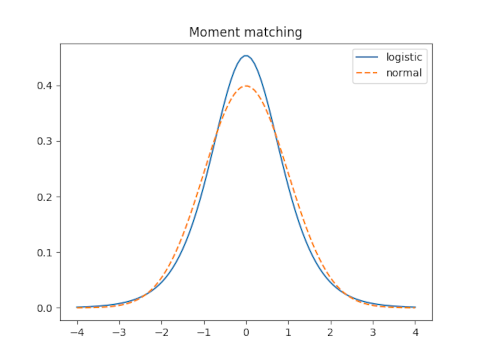
How good is this approximation? That depends on how you measure the error, which we will explore below. We will see how it compares to the optimal solution under each criterion.

1-norm

It would be nice to calculate the 1-norm of the difference f(x, s) − g(x) then minimize this as a function of s. But that difference cannot be computed in closed form. At least Mathematica can’t compute it in closed form. So I found the minimum numerically.

plot

Moment matching sets s = 0.5513 and leads to a 1-norm error of 0.1087.

The optimal value of s for the 1-norm is s = 0.6137 which yields an error of 0.0665.

2-norm

plot
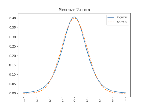
With moment matching s = 0.5513 and the 2-norm error is 0.05566.

The optimal value for the 2-norm is s = 0.61476 which yields a 2-norm error of 0.0006973.

sup-norm

The sup norm, a.k.a. min-max norm or ∞ norm, minimizes the maximum distance between the two functions.

plot

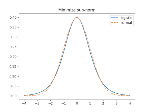
When s = 0.5513 the sup norm is 0.0545.

The optimal value of s for the sup norm is 0.6237 and yields a sup norm error of 0.01845.

Conclusion

We can improve on moment matching, for all three norms simultaneously, by using a larger value of s, such as 0.61.

If you have a normal(μ, σ) distribution and you want to approximate it by a logistic distribution, set the mean of the latter to μ and the scale to 0.61σ. If you care about a particular error measure, use the corresponding multiplier rather than 0.61.

If you want to approximate a logistic with mean μ and scale s by a normal, set the mean of the normal to μ and set σ = s/0.61.