Fax machines in the 21st century

Tens of millions of fax machines still exist. My business line gets calls from modems and fax machines fairly often. Maybe my number is close to that of a fax machine.

Fax machines and health care

Fax machines are especially common in health care. I remember when I was working at MD Anderson Cancer Center someone said IT in health care is a decade or two behind business. Still, that was a decade ago.

Fax numbers are one of the 18 things disallowed under HIPAA Safe Harbor, which is one way Safe Harbor shows its age. Few people have fax numbers anymore, but if someone does have a fax number, that could be an identifier. In fact, even knowing that someone has a fax number, without knowing what that number is, could be a privacy risk because it could help narrow down someone’s identity.

Pros and cons

There are advantages to using fax machines. You can send faxes over the internet via various services, but if you send a fax over POTS then your transmission does not go over the internet. This means the transmission is not vulnerable to some kinds of attacks, but I would think good encryption would be even better [1].

Audit trails and privacy

Fax machines either provide a better audit trail or a worse audit trail. The argument for a better audit trail is that faxes are time-stamped pieces of paper, and so are better evidence than emails. That’s one reason the legal profession likes faxes. On the other hand, once you shred a fax, it’s gone. When you delete an email, it’s hard to say how many copies of that email still exist. So faxes could be good for privacy. Maybe faxes provide a better audit trail if you want to provide an audit trail, and they make it easier to avoid an audit trail if that’s what you want.

Old technology never dies

As Kevin Kelly has pointed out, technologies never die. Of course some bizarre technologies die, but a surprising number of technologies live on, long after they’re considered obsolete. When technophiles announce that a technology is “dead”, that usually means that the technology is losing market share. A “dead” programming language, for example, may have a large and growing user base, but the user base is not growing as quickly as that of other programming languages.

Technologies are multi-faceted, and it’s rare that a new technology is better than its predecessor on every facet. The use cases for which the old technology is better occur less often over time, but if they don’t go away, the old technology won’t go away either.

Related posts

[1] Encrypted email is a mess. Encrypted email between, say, two Proton Mail accounts is secure, but email between different providers is not. An encrypted attachment is less convenient and more secure.

Blog RSS feed

I got an email from someone saying the RSS feed for this site stopped working. Anyone else having this problem?

I subscribe to my RSS feed and it’s working fine for me. It may be that there are variations on the RSS feed, and the version I’m using works while the variation some others use is not working.

I’m subscribed to

http://www.johndcook.com/blog/feed/

and that works as far as I know.

Update: The problem may have something to do with the Firefox Livemarks plugin. If you use a different RSS reader and have been having problems, please let me know.

Update: I removed one non-ASCII character from the site and that fixed at least one person’s problem with the RSS feed.

Update: Someone said changing http to https in the feed URL fixed their problem.

By the way, if you’re a blogger, I highly recommend subscribing to your own feed. Otherwise you may not know of problems. I have emailed multiple bloggers to tell them of problems with their RSS feed that they were unaware of, such as displaying LaTeX source code rather than rendered LaTeX images, for example.

***

While you’re here, let me remind you that you can find me on Mathstodon and on the platform formerly known as Twitter.

You can also subscribe to the blog or to my monthly newsletter via email.

Solitons and the KdV equation

Rarely does a nonlinear differential equation, especially a nonlinear partial differential equation, have a closed-form solution. But that is the case for the Korteweg–De Vries equation.

(Technically I should say it’s rare for a naturally-occurring nonlinear differential equation to have a closed-form solution. You can always start with a solution and cook up a contrived differential equation that it satisfies, but that differential equation will not be one that is interesting in applications.)

The Korteweg–De Vries (KdV) equation is

u_t - 6 u\, u_x + u_{xxx} = 0

This equation is used to model shallow water waves.

The KdV equation is a third-order PDE, which is unusual but not unheard of. As I wrote about earlier in the context of ODEs, third order linear equations are virtually nonexistent in application, but third order nonlinear equations are not so uncommon.

The function

u(x,t) = -\frac{v}{2} \,\text{sech}^2\left(\frac{\sqrt{v}}{2} (x - vt - a)\right )

is a solution to the KdV equation. It is an example of a class of functions known as solitons.

You can increase the amplitude by increasing v, but when you do you also increase the velocity of the wave. You can’t vary amplitude and velocity independently because the KdV equation is nonlinear.

Verifying by hand that this is a solution is tedious, so I’ll show the verification in Mathematica.

    u[x_, t_] := - (v/2) Sech[Sqrt[v] (x - v t - a)/2]^2
    Simplify[  D[u[x, t], {t, 1}]  
               - 6 u[x, t] D[u[x, t], {x, 1}] 
               + D[u[x, t], {x, 3}]  ]

This returns 0. (Without the Simplify[] command it returns a mess, but the mess simplifies to 0.)

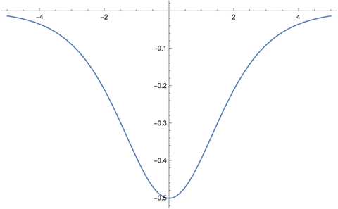
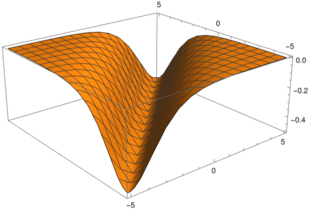
Here’s a plot of the soliton with a = 0 and v = 1.

Here’s a slice with x = 0.

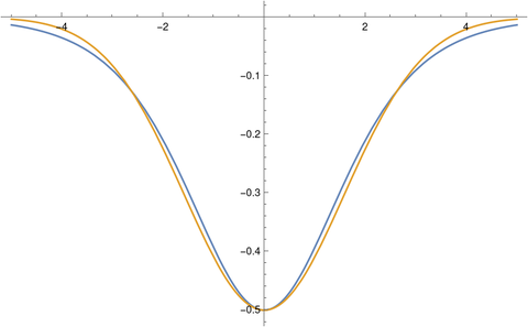
This looks remarkably like the density function of a Gaussian turned upside down. Here’s a plot with the soliton (in blue) with the density of a normal random variable with variance 5/2, scaled to have the same amplitude at 0.

Related posts

A disk around Paris

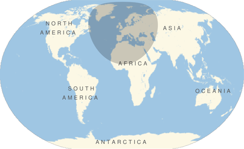
The other day I saw an image of a large disk centered on Paris subjected to the Mercator projection. I was playing around in Mathematica and made similar images for different projections. Each image below is a disk of radius 4200 km centered on Paris (latitude 49°, longitude 2°).

All images were produced with the following Mathematica code, changing the GeoProjection argument each time.

    GeoGraphics[GeoDisk[GeoPosition[{49, 2}],
       Quantity[4200, "Kilometers"] ],
       GeoProjection -> "...", 
       GeoRange -> "World"]

Robinson projection

    … GeoProjection -> "Robinson", …

Robinson projection

Winkel-Snyder projection

    … GeoProjection -> "WinkelSnyder", …

Winkel-Snyder projection

Orthographic projection

    … GeoProjection -> "Orthographic", …

Orthographic projection

Lambert Azimuthal projection

    … GeoProjection -> "LambertAzimuthal", …

Lambert Azimuthal projection

Peirce Quincuncial projection

    … GeoProjection -> "PeirceQuincuncial", …

Peirce Quincuncial projection

This last projection has some interesting mathematics and history behind it. See this post for the backstory.

Using classical statistics to avoid regulatory burden

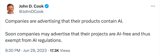
On June 29 this year I said on Twitter that companies would start avoiding AI to avoid regulation.

Companies are advertising that their products contain AI. Soon companies may advertise that their projects are AI-free and thus exempt from AI regulations.

I followed that up with an article Three advantages of non-AI models. The third advantage I listed was

Statistical models are not subject to legislation hastily written in response to recent improvements in AI. The chances that such legislation will have unintended consequences are roughly 100%.

Fast forward four months and we now have a long, highly-detailed executive order, Executive Order 14110, effecting all things related to artificial intelligence. Here’s an excerpt:

… the Secretary [of Commerce] shall require compliance with these reporting requirements for: any model that was trained using a quantity of computing power greater than 1026 integer or floating-point operations, or using primarily biological sequence data and using a quantity of computing power greater than 1023 integer or floating-point operations; and any computing cluster that has a set of machines physically co-located in a single datacenter, transitively connected by data center networking of over 100 Gbit/s, and having a theoretical maximum computing capacity of 1020 integer or floating-point operations per second for training AI.

If a classical model can do what you need, you are not subject to any regulations that will flow out of the executive order above, not if these regulations use definitions similar to those in the executive order.

How many floating point operations does it take to train, say, a logistic regression model? It depends on the complexity of the model and the amount of data fed into the model, but it’s not 1020 flops.

Can you replace an AI model with something more classical like a logistic regression model or a Bayesian hierarchical model? Very often. I wouldn’t try to compete with Midjourney for image generation that way, but classical models can work very well on many problems. These models are much simpler—maybe a dozen parameters rather than a billion parameters—and so are much better understood (and so there is less fear of such models that leads to regulation).

I had a client that was using some complicated models to predict biological outcomes. I replaced their previous models with a classical logistic regression model and got better results. The company was so impressed with the improvement that they filed a patent on my model.

If you’d like to discuss whether I could help your company replace a complicated AI model with a simpler statistical model, let’s talk.

Executive order on differential privacy

US whitehouse

This week President Biden signed a long, technically detailed executive order (Executive Order 14110) that among other things requires the Secretary of Commerce to look into differential privacy.

Within 365 days of the date of this order … the Secretary of Commerce … shall create guidelines for agencies to evaluate the efficacy of differential-privacy-guarantee protections, including for AI. The guidelines shall, at a minimum, describe the significant factors that bear on differential-privacy safeguards and common risks to realizing differential privacy in practice.

I doubt many people have read this order. Print preview on my laptop said it would take 64 pages to print. Those brave souls who try to read it will find technical terms like differential privacy that they likely do not understand.

So just what is differential privacy? A technical definition involves bounds on ratios of cumulative probability distributions functions, not the kind of thing you usually see in newspapers, or in executive orders.

I’ll give a layman’s overview here. If you’d like to look at the mathematical details, see this post for a gentle introduction. And if you want even more math, see this post.

What is differential privacy?

The basic idea behind differential privacy is to protect the privacy of individuals represented in a database by limiting the degree to which each person’s presence in the database can impact queries of the database.

A calibrated amount of randomness is added to the result of each query. The amount of randomness is proportional to the sensitivity of the query. For innocuous queries the amount of added randomness may be very small, maybe even less than the amount of uncertainty inherent in the data. But if you ask a query that risks revealing information about an individual, the amount of added randomness increases, possibly increasing so much that the result is meaningless.

Each question (database query) potentially reveals some information about a person, and so a privacy budget keeps track of the queries a person has posed. Once you’ve used up your privacy budget, you’re not allowed to ask any more questions. Otherwise you could ask the same question (or closely related questions) over and over, then average your results to essentially remove the randomness that was added.

Pragmatic matters

Differential privacy is great in theory, and possibly in practice too. But the practicality depends a great deal on context. For example, exactly how much noise is added to query results? That depends on the level of privacy you want to achieve, usually denoted by a parameter ε. Smaller values of ε provide more privacy, and larger values provide less.

How big should ε be? There is no generic answer. The size of ε must depend on context. Set ε too small and the utility of the data vanishes. Set ε too high and there’s effectively no privacy protection.

US Census Bureau

Biden’s executive order isn’t the US government forey into differential privacy. The US Census Bureau used differential privacy on results released from the 2020 census. This means that the reported results are deliberately not accurate, though hopefully the results are accurate enough, with only the minimum amount of inaccuracy injected as necessary to preserve privacy. Opinions are divided on whether that was the case. Some researchers have complained that the results were too noisy for the data they care about. The Census Bureau could reply “Sorry, but we gave you the best results we could while adhering to our privacy framework.”

Implementing differential privacy at the scale of the US Census took an enormous amount of work. The census serves as a case study that would allow other government agencies to have an idea of what they’re getting into.

Pros and cons of differential privacy

Differential privacy rests on a solid mathematical foundation. While this means that it provides strong privacy guarantees (if implemented correctly), it also means that it takes some effort to understand. Differential privacy opens up new possibilities but requires new ways of working.

If you’d like help understanding how your company could take advantage of differential privacy, or minimize the disruption of being required to implement differential privacy, let’s talk.

Related posts

Differential entropy and privacy

Differential entropy is the continuous analog of Shannon entropy. Given a random variable X with density function fX, the differential entropy of X, denoted h(X), is defined as

h(X) = -\int f_X(x) \log_2 f_X(x)\, dx

where the integration is over the support of fX. You may see differential entropy defined using logarithm to a different base, which changes h(X) by a constant amount.

In [1] the authors defined the privacy of a random variable X, denoted Π(X), as 2 raised to the power h(X).

\Pi(X) = 2^{h(X)}

This post will only look at “privacy” as defined above. Obviously the authors chose the name because of its application to privacy in the colloquial sense, but here we will just look at the mathematics.

Location and scale

It follows directly from the definitions above that location parameters do not effect privacy, and scale parameters change privacy linearly. That is, for σ > 0,

\Pi(\sigma X + \mu) = \sigma \,\Pi(X)

If we divide by standard deviation before (or after) computing privacy then we have a dimensionless quantity. Otherwise there’s more privacy is measuring a quantity in centimeters than in measuring it in inches, which is odd since both contain the same information.

Examples

If X is uniformly distributed on an interval of length a, then h(X) = log2 a and Π(X) = a.

The privacy of a standard normal random variable Z is √(2πe) and so the privacy of a normal random variable with mean μ and variance σ² is σ√(2πe).

The privacy of a standard exponential random variable is 1, so the privacy of an exponential with rate λ is 1/λ.

Bounds

A well-known theorem says that for given variance, differential entropy is maximized by a normal random variable. This means that the privacy of a random variable with variance σ² is bounded above by σ√(2πe).

The privacy of a Cauchy random variable with scale σ is 4πσ, which is greater than σ√(2πe). This is does not contradict the statement above because the scaling parameter of a Cauchy random variable is not its standard deviation. A Cauchy random variable does not have and standard deviation.

Related posts

[1] Agrawal D., Aggrawal C. C. On the Design and Quantification of Privacy-Preserving Data Mining Algorithms, ACM PODS Conference, 2002. (Yes, the first author’s name contains one g and the second author’s name contains two.)

Positive polynomials revisited

The square of a real-valued polynomial is clearly non-negative, and so the sum of the squares of polynomials is non-negative. What about the converse? Is a non-negative polynomial the sum of the squares of polynomials?

For polynomials in one variable, yes. For polynomials in several variables, no.

However, Emil Artin proved nearly a century ago that although a non-negative polynomial cannot in general be written as a sum of squares of polynomials, a non-negative polynomial can be written as a sum of squares of rational functions.

Several years ago I wrote about Motzkin’s polynomial,

M(x,y) = x^4 y^2 + x^2 y^4 + 1 - 3x^2 y^2

an explicit example of a non-negative polynomial in two variables which cannot be written as the sum of the squares of polynomials. Artin’s theorem says it must be possible to write M(x, y) as the sum of the squares of rational functions. And indeed here’s one way:

\begin{align*} M(x,y) &= x^4 y^2 + x^2 y^4 + 1 - 3x^2 y^2 \\ &= \left( \frac{x^2y(x^2 + y^2 - 2)}{x^2 + y^2} \right)^2 + \left( \frac{xy^2(x^2 + y^2 - 2)}{x^2 + y^2} \right)^2 + \\ &\phantom{=} \,\,\, \left( \frac{xy(x^2 + y^2 - 2)}{x^2 + y^2} \right)^2 + \left( \frac{x^2 - y^2}{x^2 + y^2} \right)^2 \end{align*}

Source: Mateusz Michaelek and Bernd Sturmfels. Invitation to Nonlinear Algebra. Graduate Studies in Mathematics 211.

Here’s a little Mathematica code to verify the example above.

m[x_, y_] := x^4 y^2 + x^2 y^4 + 1 - 3 x^2 y^2
a[x_, y_] := (x y (x^2 + y^2 - 2))/(x^2 + y^2)
b[x_, y_] := (x a[x, y])^2 + (y a[x, y])^2 + a[x, y]^2 
             + ((x^2 - y^2)/(x^2 + y^2))^2
Simplify[m[x, y] - b[x, y]]

This returns 0.

Identifiers depend on context

Can you tell who someone is from their telephone number? That’s kinda the point of telephone numbers, to let you contact someone. And indeed telephone number is one the 18 identifiers under HIPAA Safe Harbor.

But whether any piece of information allows you to identify someone depends on context. If you don’t have access to a phone, or a phone book, or any electronic counterpart of a phone book, then a phone number doesn’t allow you to identify anyone. But once you can call a phone number or enter it into a search engine, then the phone number is identifiable. Maybe.

What if the number belongs to a burner phone? Then it would be harder to learn the identity of the person who owns the number, but not impossible. Maybe you couldn’t learn anything about the owner, but law enforcement officials could. Again identifiability depends on context.

An obvious identifier like a phone number might not be an identifier in some special circumstance. And an apparently useless bit of information might reveal someone’s identity in another circumstance.

HIPAA’s Safe Harbor Rule tries to say apart from context what kinds of data are identifiable. But if you read the Safe Harbor Rule carefully you’ll notice it isn’t so context-free as it seems. The last item in the list of 18 items to remove is “any other unique identifying number, characteristic, or code.” What might be an identifying characteristic? That depends on context.

Country and language abbreviations

I recently had to mark a bit of German text as German in an HTML file and I wondered whether the abbreviation might be GER for German, or DEU for deutsche.

Turns out the answer is both, almost. The language abbreviations used for HTML microdata are given in ISO 639, and they come in three-letter and two-letter varieties. The three-letter abbreviation for German is GER but the two-letter abbreviation is DE.

There are also standard two- and three-letter abbreviations for countries, given in ISO 3166. These are DE and DEU for Germany. I was curious how often a country abbreviation is also a language abbreviation.

I found text files giving the ISO 639 and ISO 3166 abbreviations, and used the comm utility to see how what the intersection was.

There are 253 languages and 252 countries in the two standards. There are 110 two-letter abbreviations common to both, and 40 three-letter abbreviations common to both.

However, just because an abbreviation appears in both standards, this doesn’t mean it represents the same thing in both standards. Sometimes they overlap. For example CZE abbreviates both the Czech Republic and the Czech language. But BEL represents the nation of Belgium and the Belarusian language.