cos(200!)

In a footnote to the previous post, I said that Python’s math library can calculate the logarithm of extremely large numbers but not the cosine. This post will expand on that comment.

In this post I’ll use n = 200! as my example rather than 1000! because this value of N is larger than the largest representable floating point number but small enough to be more convenient to work with.

Suppose someone calculates 200! for you:

78865786736479050355236321393218506229513597768717326329474253324435\
94499634033429203042840119846239041772121389196388302576427902426371\
05061926624952829931113462857270763317237396988943922445621451664240\
25403329186413122742829485327752424240757390324032125740557956866022\
60319041703240623517008587961789222227896237038973747200000000000000\
00000000000000000000000000000000000

You could now calculate log(n) using

n = 7.886578673647905 × 10374

and so

log(n) = log(7.886578673647905 × 10374)
= log(7.886578673647905) + 374 log(10) = 863.2319871924055.

The key thing that makes this possible is that the least significant digits of n only affect the least significant digits of log(n). In the calculation above I kept the first 16 digits of n. Python couldn’t make use of any more digits, and had no need of any more digits, in order to produce the logarithm to machine precision.

Cosine doesn’t work that way. The cosine of n depends on the remainder when n is divided by 2π, and that remainder depends on every single digit of n. I’ll illustrate that below.

Using bc -l and setting the scale to 400, I can calculated n then calculate

cos(n + 10i)

for i running from 0 to 374, tweaking each digit one at a time. (Except when a digit is a 9 and the addition results in a carry.)

    n = 1
    for (i = 1; i <= 200; i++) n *= i
    scale = 400
    for (i = 1; i <= 374; i++) {
        x = c(n+10^i)
        scale = 16
        print x/1, "\n"
        scale = 400
    }

Here’s what a plot of the results look like.
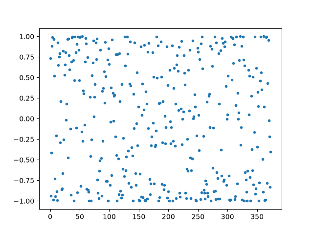
The value of cos(n) is about −0.985, but the values above are all over the map. We can look at the range by projecting all the points over to the left edge then rotating a quarter turn:

The remarkable thing about this image is that there are a few gaps, i.e. a few values the cosine does not take on.

Here’s a more sophisticated way to look at it. The sequence 10i mod 2π is dense in [0, 2π], and so by going far enough out in the sequence, we can find a value that shifts the phase of n by any desired amount within any given tolerance.

Every digit in n matters, and changing any digit can change the value of cosine to be essentially any value. You cannot calculate the cosine of an enormous number without using some kind of extended precision arithmetic. There are clever range reduction algorithms that minimize the amount of extended arithmetic necessary, but extended arithmetic cannot be completely eliminated.
Calculating log(1000!)

The previous post pointed out that the following code such as the following unexpectedly works.

>>> from math import log, factorial
>>> log(factorial(1000))
5912.128178488163

If you don’t find this unexpected, note that if you replace math.log with numpy.log the code will fail [1]. Functions like natural logarithm operate on real numbers. Real numbers are represented as floating point numbers in programming languages, and 1000! factorial is too large to represent as a standard floating point number. (More on that here.)

In this post I’d like to look at how you might calculate log(1000!) with less capable software, and even without software.

One approach would be to sum the logarithms of the numbers 1 through 1000. This will give essentially the same result as above, with a little difference in the last couple decimal places due to rounding error.

If you have a way to calculate 1000! but not a way to cast it to a floating point number, you could do this manually.

>>> s = str(factorial(1000))
>>> s[:16]
'4023872600770937'
>>> len(s)
2568

This tells us 1000! = 4.023872600770937 × 102567. Therefore

log(1000!) = log(4.023872600770937) + 2567 log(10)

which only requires working with numbers of modest size.

Calculating by hand

Now suppose it’s 1964. You don’t have a computer, or even a calculator, but you do have a copy of the recently published Handbook of Mathematical Functions by Abramowitz and Stegun (A&S). You turn to Table 6.6 “Factorials for large arguments.” This has values of factorial for 100, 200, 300, …, 1000, so you can simply look up your answer to 20 decimal places.

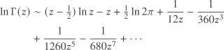
That was too easy; I didn’t expect that to be there when I started writing this post. If you wanted to compute log(950!), for example, you’d have to work harder. You could find A&S equation 6.1.41 (Stirling’s series) which says

\begin{align*} \ln \Gamma(z) &\sim (z - \tfrac{1}{2}) \ln z - z + \tfrac{1}{2} \ln 2\pi + \frac{1}{12z} - \frac{1}{360z^3} \\ &+ \frac{1}{1260z^5} - \frac{1}{680z^7} + \cdots \end{align*}

So how would you use this formula to calculate log(1000!)? Since n! = Γ(n + 1), you set z = 1001.

You’d need to decide how many terms you need to use. Assuming the error is on the order of the first term you leave out, you’d reason that you could probably stop with the 1/12z term because the next term is between 10−11 and 10−12.

You find Table 4.2 has natural logarithms, but not for 1001. You can look up log(1.001), however, and at the bottom of the same page is log(10) to 16 decimal places, and you can find log(10) to 24 decimal places in Table 1.1. So you calculate

log(1001) = log(1.001 × 10³) = log(1.001) + 3 log(10).

You can find log(2) and log(π) in Table 1.1, and average them to find ½ log(2π).

Here’s Python code to simulate the hand calculations.

log2     = 0.6931_47180_55994_53094_172321 # Table 1.1
log10    = 2.3025_85092_99404_56840_179915 # Table 1.1
logpi    = 1.1447_29885_84940_01741_43427  # Table 1.1
log1_001 = 0.00099_95003_330835            # Table 4.2

z = 1001
logz = log1_001 + 3*log10
s = (z - 0.5)*logz - z + (log2 + logpi)/2 + 1/(12*z)

print(s)

This result differs from the one at the top of the post only in the last decimal place.

Related posts

Doing calculations with tables is not as simple as “just look it up.” It takes a bit of skill.

[1] The code will also fail if you replace math.log with math.cos. Both logarithm and cosine return moderate sized real numbers when given enormous inputs like 1000!, so representing the output as a float is not the problem. But logarithms of huge numbers can be computed with ordinary precision functions, as above. But computing the cosine of a huge number requires extended precision.

Update: The next post expands on why computing the cosine of a large number is more difficult than computing the log.

The code that didn’t break

Last week I wrote a post on hiding cryptographic keys in decks of cards. I wrote some code for that post that shouldn’t work, but before fixing I noticed that it in fact did work.

The code computes logarithms for integers larger than the largest representable float. For example, the largest float is on the order of 10308, and yet the following code works.

>>> import math
>>> math.log10(10**400)
400.0

The log, log2, and log10 functions have some code inside that handles large integers specially. It doesn’t simply convert the integers to floats before taking the logarithm. If it did, it would overflow. If you replace math with numpy above, the code will fail. NumPy’s implementation of logarithms is more what I would expect.

While playing around with this I also noticed that you can define floats larger than the largest float without warnings.

>>> math.log(1e308)
709.1962086421661
>>> math.log(1e309)
inf

This isn’t a feature of math.log but of how Python handles scientific notation. The expression 1e308 is the floating point representation of 10308. It is a float, not an int.

>>> type(1e308)
<class 'float'>

The expression 1e309 is also a float. But since it’s larger than is possible for a float, Python interprets it as inf. The code

math.log(1e309)

returns inf based on the reasoning that log(∞) = ∞.

That explains the following behavior:

>>> 1e309 == 1e310
True

The expressions 1e309 and 1e310 are equal because both are alternate ways of writing inf.

Enumerating trees and circles

A few days ago I wrote a post on counting rooted trees. That post looked at the sequence c(n) which counts the number of rooted trees with n nodes. Here one node is distinguished as the root, but the nodes below the root are not distinguished from each other; all that matters is how the nodes are connected.

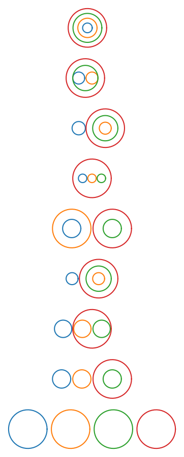
The number of rooted trees with n nodes is the same as the number of ways to configure n − 1 non-overlapping circles. Not only are the counts the same, there is a natural correspondence between the trees and the circles. It’s not obvious that there should be such a correspondence, with the right notation the correspondence is sort of a pun.

The standard way to represent unlabeled trees is as a multiset of their children. We use a multiset, not a set, because some elements will be repeated. We represent a leaf as a pair of parentheses: ().

There is only one rooted tree with one node: ().

There is only one rooted tree with one two nodes: (()). Here the outer parentheses represent the root node and the inner parentheses represent its child.

There are two rooted trees with three nodes, and we can represent them as ((())) and ((),()). The first is the straight line tree: a node that has a single child node that has a single child node. The second is a node that branches to two nodes. (Here’s where we need multisets.)

The four rooted trees with four nodes can be represented as (((()))), ((((),())), ((),(())), and ((),(),(),()).

Here are the nine rooted trees with five nodes:

((((()))))
((((),())))
(((),(())))
(((),(),()))
((()),(()))
((),((())))
((),((),()))
((),(),(()))
((),(),(),())

The correspondence with non-overlapping circles removes the outer parentheses then joins the rest to form circles, with nested parentheses corresponding to concentric circles. A more geometric way to see the correspondence is to start at the bottom of the tree, replace leaves with circles, then work your way up circling connected components.

Mathematical alchemy

After writing the previous post about metallic ratios, I thought about the analogy to alchemy and the attempt to make precious metals out of base metals.

When can you make one metallic ratio out of another? Can you make the golden ratio out of the lead ratio?

Before we can make gold out of lead, we have to say what lead is.

Defining metallic ratios

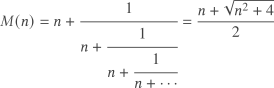
The metallic ratios M(n) can be defined several ways. The most interesting definition is the number whose continued fraction representation contains all ns. A more prosaic but more convenient definition is the larger number that equals its reciprocal plus n, which can be found using the quadratic formula.

M(n) = n + \cfrac{1}{n+\cfrac{1}{n+\cfrac{1}{n+\cdots}}} = \frac{n + \sqrt{n^2 + 4}}{2}

The golden ratio is M(1), the silver ratio is M(2), and the bronze ratio is M(3).

Gold from silver and bronze?

Can you make the golden ratio out of the silver and bronze ratios? Not by integer arithmetic. The golden ratio involves √5, the silver ratio √2 and the bronze ratio √13. No integer operations on the latter two radicals will produce the former, though you can come arbitrarily close.

Gold from lead

The metallic ratios for n > 3 don’t have standard names, but let’s call M(4) the lead ratio. Can you make the golden ratio out of the lead ratio? Yes you can:

M(1) = (M(4) − 1)/2.

General solution

In general, when can you make M(n) out of M(m)? In abstract terms the question is when the fields

ℚ(√(n² + 4))

and

ℚ(√(m² + 4))

are the same, i.e. when adjoining √(n² + 4) to the rational numbers gives the same field as adjoining √(m² + 4) to the rational numbers. This occurs if and only if

(n² + 4)/( + 4)

is the square of a rational number.

Bronze from copper and tin

Can you make bronze out of copper and tin? Yes, if you define M(36) to be the copper ratio and M(393) to be the tin ratio, because

(3² + 4)/(36² + 4) = (1/10)²

and

(3² + 4)/(292² + 4) = (1/109)².

Ratio of metallic ratios

The golden ratio is the first and best known of the metallic ratios. I’ve written about the silver ratio a few times, most recently here. And I’ve mentioned the bronze ratio a couple times. The metallic ratios after bronze don’t have standard names.

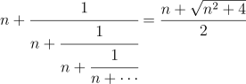
The nth metallic ratio M(n) is the number whose continued fraction representation contains all ns.

n + \cfrac{1}{n+\cfrac{1}{n+\cfrac{1}{n+\cdots}}} = \frac{n + \sqrt{n^2 + 4}}{2}

When n = 1, 2, and 3 we get the gold, silver, and bronze ratios.

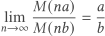
You can approximate any positive real number as a ratio of metallic ratios. To see this, note that for large n, M(n) is approximately n. For any positive rational number a/b,

\lim_{n\to\infty} \frac{M(na)}{M(nb)} = \frac{a}{b}

and so you can make M(na) / M(nb) as close to a/b as you like by taking n large enough. And since the rationals are dense in the reals, you can approximate any positive real number as close as you’d like.

Let’s look for metallic ratios whose ratios approximate π to within 0.001 with the following Python code.

from math import pi, sqrt

M = lambda n: 0.5*(n + sqrt(n**2 + 4))

for n in range(1, 100):
    a = round(pi*n)
    b = n
    r = M(a)/M(b)
    if abs(r - pi) < 0.001:
        print(a, b, r)

This shows

π ≈ M(132) / M(42) = 3.1412…

Could we find smaller numbers that work? The following code shows the answer is no.

k = 132 + 42
# loop over numbers whose sum is less than k
for n in range(1, k):
    for a in range(1, n):
        b = n - a
        r = M(a)/M(b)
        if abs(r - pi) < 0.001:
            print(a, b, r)
            exit()

Related posts

Holonomic functions

Yesterday I wrote that a lot of the special functions that pop up in mathematical physics are solutions to second order linear differential equations with polynomial coefficients. More generally, holonomic functions are defined to be those functions that are the solutions to linear differential equations, of any order, with polynomial coefficients.

Most special functions are holonomic. To quantify that statement, I went through the special functions covered in Abramowitz and Stegun. The large majority are holonomic, though some common functions like the gamma function are not holonomic.

This report goes through the functions in A&S. For those that are holonomic, it gives the differential equation that the function solves. The large majority of these equations are second order, but not all. And the coefficients are nearly always first or second order polynomials, rarely higher order.

Estimating a cumulative sum

In this post I mentioned two series which I denoted t(n) and c(n). The former is the number of unlabeled rooted trees with n nodes. The latter is the cumulative sum of the former, i.e.

c(n) = t(1) + t(2) + t(3) + \cdots + t(n)

The sequence c(n) is also the number of constraints on an n-step Runge-Kutta method; that’s how I became interested in it.

Now the t(n) sequence has been cataloged as OEIS A000081 and OEIS gives the asymptotic estimate of t(n) for large n as

t(n) \sim C \frac{a^n}{n^{3/2}}

where C = 0.4399… and α = 2.9557….

The cumulative sum of t(n), what I’ve called c(n), is also cataloged in OEIS, sequence number A087803. However, OEIS does not give an asymptotic estimate for this sequence. I’ll give one here.

(Update: After looking closer at the page for A087803 I see that there is an asymptotic formula, the same one derived here.)

The basis for my derivation is to assume the cumulative sum of the asymptotic estimates gives an asymptotic estimate of the cumulative sum. This is justified by the fact that the sequence is increasing rapidly and only the last few terms contribute much relatively to the sum.

The technique illustrated here would be applicable to the cumulative sum of other series whose asymptotic form is known.

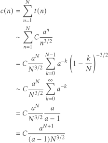
\begin{align*} c(n) &= \sum_{n=1}^N t(n) \\ &\sim \sum_{n=1}^N C \frac{a^n}{n^{3/2}}\\ &= C \frac{a^N}{N^{3/2}} \sum_{k=0}^{N-1} a^{-k}\left(1 - \frac{k}{N} \right)^{-3/2} \\ &\sim C \frac{a^N}{N^{3/2}} \sum_{k=0}^\infty a^{-k} \\ &= C \frac{a^N}{N^{3/2}} \frac{a}{a-1} \\ &= C \frac{a^{N+1}}{(a-1)N^{3/2}} \end{align*}

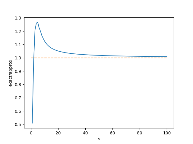
Here’s code to visualize the rate of convergence.

import numpy as np
import matplotlib.pyplot as plt

# from https://oeis.org/A000081/b000081.txt
A000081 = [
    0,
    1,
    1,
    2,
    4,
    ...
    51384328351659326880337136395054298255277970,
]  
A087803 = np.cumsum(A000081)

def approx(n):
    C = 0.43992401257102530
    a = 2.95576528565199497
    return C*a**(n+1)*n**(-3/2)/(a - 1)

n = np.arange(len(A087803))
ratio = A087803/approx(n)

plt.plot(n[1:], ratio[1:])
plt.plot(n, 0*n + 1, '--')
plt.xlabel("$n$")
plt.ylabel("exact/approx")
plt.show()

Here’s the plot:

Why polynomial coefficients?

Second order linear differential equations with polynomial coefficients form their own area of study. This seems like a narrow class of equations, but it’s very important in applications.

This class of equations seems like a mathematically natural topic, but why is it so important in applications? I did a PhD in differential equations without ever learning why. The theory of second order linear equations with polynomial coefficients is too complicated for undergraduate courses [0] and too well-established for graduate courses [1].

The explanation that I was missing can be found in the first chapter of [2]. The PDEs that are common in physics are separable in various coordinate systems, meaning that in these coordinate systems the PDEs reduce to ODEs. These ODEs either have polynomial coefficients, or there is a change of variables which makes the ODEs have polynomial coefficients.

See this writeup that looks at the Helmholtz and Laplace equations in 11 coordinate systems.

[0] You may see the simplest parts of the theory in a section on solving ODEs with power series. But textbooks don’t go very far for good reasons.

[1] Unfortunately, a lot of really useful topics are left out of the graduate curriculum because they’re too well understood to provide thesis topics. Or the problems that are still open have been open for so long that they’re likely too hard to be cracked by a graduate student.

[2] Gerhard Kristensson. Second Order Differential Equations: Special Functions and their Classification. Springer, 2010.

Counting rooted trees

Combinatorial problems can be interesting for their own sake, but they are more interesting when there is a connection to a problem outside combinatorics, and the more unexpected the connection the better.

Counting the number of unlabeled rooted trees [1] with n nodes is a pure mathematics problem. Designing numerical methods for solving differential equations is an applied mathematics problem. And yet the two are closely linked.

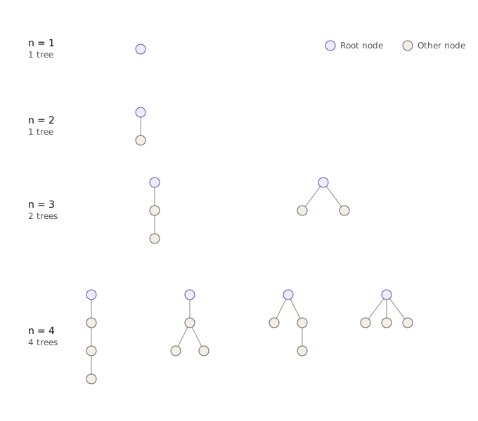
Let t(n) be the number of distinct unlabeled rooted trees with n nodes. The diagram below shows that the first few terms of this sequence are 1, 1, 2, and 4.

Recursive calculation

The values of t(n) can be computed recursively using

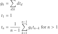
\begin{align*} g_k &= \sum_{d\mid k} d t_d \\ t_1 &= 1 \\ t_n &= \frac{1}{n-1} \sum_{k=1}^{n-1} g_k t_{n-k} \text{ for } n > 1<br />
\end{align*}<br />

You can implement this in Python as follows.

from sympy import divisors

def t(n):
    if n <= 1:
        return 1 if n == 1 else 0
    return sum(g(k) * t(n - k) for k in range(1, n)) // (n - 1)

def g(k):
    return sum(d * t(d) for d in divisors(k))

This code is correct, but it will run more efficiently if you cache function values to avoid calculating the same values over and over. You can do this by adding

from functools import lru_cache

and writing @lru_cache(maxsize=None) above both function definitions.

Connection to Runge-Kutta

In an earlier post I showed that designing a 4-stage explicit Runge-Kutta method required solving a system of 8 equations in 10 unknowns, leaving two degrees of freedom in the solutions.

The number of constraints c(s) needed to design an s-stage explicit RK method is equal to the number of rooted trees with up to s nodes:

c(s) = t(1) + t(2) + t(3) + … + t(s)

This is because there is a one-to-one correspondence between constraints on the nth derivative of an RK formula and rooted trees, and an s stage method has to satisfy the constraints of all stages up to s. In the example of the 4th order RK method, we have

c(4) = t(1) + t(2)  + t(3) + t(4) = 1 + 1 + 2 + 4 = 8.

The first few values [2] of t(n) are

1, 1, 2, 4, 9, 20, 48, 115, 286, 719, 1842, 4766, 12486, 32973, …

and so you can see that t(n) grows quickly. In fact, it grows exponentially [3].

However, the number of parameters in an s stage RK method is s(s + 1)/2. The number of equations grows exponentially and the number of variables grows only quadratically, so at some point you have more equations than variables. That’s already the case for s = 5 because you have 17 constraints on 15 variables. The system has a solution because symmetry considerations render some of the equations redundant.

A 10th order RK method requires 17 stages. (See the previous post for why the number of stages exceeds the order when the order is greater than 4.) Designing such a method would require solving over a million equations in 153 variables, and yet it can be done. [4]

Related posts

[1] This is a slightly contradictory term. Unlabeled means the we don’t distinguish the nodes. But we do distinguish one node, namely the root.

[2] See OEIS A000081.

[2] Richard Otter proved in 1948 that the number of unlabeled rooted trees with n nodes is asymptotically C αn / n−3/2 where C = 0.4399… and α = 2.9557…. The cumulative sum is at least this large since Otter’s estimate gives the size of the last term in the sum.

[3] E. Hairer. A Runge-Kutta Method of Order 10. J. Inst. Maths Applics (1978) 21, 47-59