I’ve written a couple posts lately about reverse engineering the internal state of a random number generator, first Mersenne Twister then lehmer64. This post will look at xorshift128, implemented below.
import random

# Seed the generator state
a: int = random.getrandbits(32)
b: int = random.getrandbits(32)
c: int = random.getrandbits(32)
d: int = random.getrandbits(32)

MASK = 0xFFFFFFFF

def xorshift128() -> int:
    global a, b, c, d

    t = d
    s = a

    t ^= (t << 11) & MASK t ^= (t >>  8) & MASK
    s ^= (s >> 19) & MASK

    a, b, c, d = (t ^ s) & MASK, a, b, c

    return a
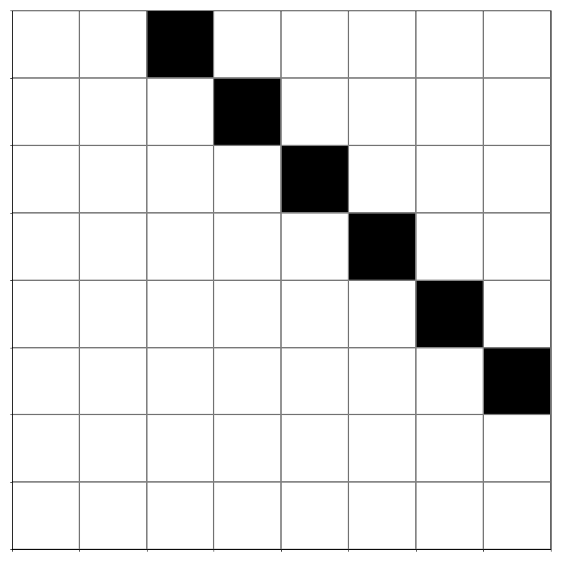
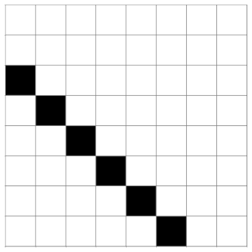
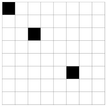
Recovering state
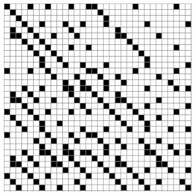
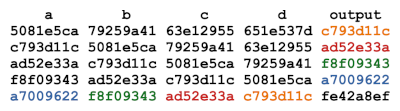
Recovering the internal state of the generator is simple: it’s the four latest outputs in reverse order. This is illustrated by the following chart.
This means that once we’ve seen four outputs, we can predict the rest of the outputs. The following code demonstrates this.
Let’s generate five random values.
out = [xorshift128() for _ in range(5)]
Running
print(hex(out[4]))
shows the output 0xc3f4795d.
If we reset the state of the generator using the first four outputs
d, c, b, a, _ = out
print(hex(xorshift128()))
we get the same result.
Good stats, bad security
Mersenne Twister and lehmer64 have good statistical properties, despite being predictable. The xorshift128 generator is even easier to predict, but it also has good statistical properties. These generators would be fine for many applications, such as Monte Carlo simulation, but disastrous for use in cryptography.
The post on lehmer64 mentioned at the end that the internal state of PCG64 can also be recovered from its output. However, doing so requires far more sophisticated math and thousands of hours of compute time. Still, it’s not adequate for cryptography. For that you’d need a random number generator designed to be secure, such as ChaCha.
So why not just use a cryptographically secure random number generator (CSPRNG) for everything? You could, but the other generators mentioned in this post use less memory and are much faster. PCG64 occupies an interesting middle ground: simple and fast, but not easily reversible.