Solving hard problems

We help companies solve hard problems in mathematics, statistics, and computing. Let’s explore how we might work together.

Solving equations with Lambert’s W function

Posted on 14 November 2021 by John

In the previous post we wanted to find a value of n such that f(n) = 10¹² where

$f(n) = \frac{1}{4n\sqrt{3}} \exp\left( \pi \sqrt{\frac{2n}{3}} \right)$

and we took a rough guess n = 200. Turns out f(200) ≈ 4 × 10¹² and that was good enough for our purposes. But what if we wanted to solve f(n) = x accurately?

We will work our way up to solving f(n) = 10¹² exactly using the Lambert W function.

Lambert’s W function

If you can solve one equation involving exponential functions you can bootstrap your solution solve a lot more equations.

The Lambert W function is defined to be the function W(x) that maps each x to a solution of the equation

w exp(w) = x.

This function is implemented Python under scipy.special.lambertw. Let’s see how we could use it solve similar equations to the one that define it.

Basic bootstrapping

Given a constant c we can solve

cw exp(w) = x

simply by solving

w exp(w) = x/c,

which says w = W(x/c).

And we can solve

w exp(cw) = x

by setting y = cw and solving

y exp(y) = cx.

and so cw = W(cx) and w = W(cx)/c.

Combining the two approaches above shows that the solution to

aw exp(bw) = x

w = W(bx/a) / b.

We can solve

exp(w) / w = x

by taking the reciprocal of both sides and applying the result above with a = 1 and b = -1.

More generally, we can solve

w^c exp(w) = x

by raising both sides to the power 1/c; the reciprocal the special case c = 1.

Similarly, we can solve

w exp(w^c) = x

by setting y = w^c , changing the problem to

y^-1/c exp(y) = x.

Putting it all together

We’ve now found how to deal with constants and exponents on w, inside and outside the exponential function. We now have all the elements to solve our original problem.

We can solve the general equation

$a w^b \exp(c w^d) = x$

with

$w = \left(\frac{b}{cd} \,\,W\left(\frac{cd}{b} \left(\frac{x}{a} \right )^{d/b} \right )\right )^{1/d}$

The equation at the top of the post corresponds to a = 1/√48, b = -1, c = π √(2/3), and d = 1/2.

We can code this up in Python as follows.

    from scipy.special import lambertw

    def soln(a, b, c, d, x):
        t = (x/a)**(d/b) *c*d/b
        return (lambertw(t)*b/(c*d))**(1/d)

We can verify that our solution really is a solution by running it though

    from numpy import exp, pi

    def f(a, b, c, d, w):
        return a*w**b * exp(c*w**d)

to make sure we get our x back.

When we run

    a = 0.25*3**-0.5
    b = -1
    c = pi*(2/3)**0.5
    d = 0.5
    x = 10**12

    w = soln(a, b, c, d, x)
    print(f(a, b, c, d, w))

we do indeed get x back.

    a = 0.25*3**-0.5
    b = -1
    c = pi*(2/3)**0.5
    d = 0.5

    w = soln(a, b, c, d, 10)
    print(f(a, b, c, d, w))

When we take a look at the solution w, we get 1.443377079584187e-13. In other words, we get a number near zero. But our initial guess was w = 200. What went wrong?

Nothing went wrong. We got a solution to our equation. It just wasn’t the solution we expected.

The Lambert W function has multiple branches when viewed as a function on complex numbers. It turns out the solution we were expecting is on the branch SciPy denotes with k = -1. If we add this to the call to lambertw above we get the solution 183.85249773880142 which is more in line with what we expected.

Estimating the number of integer partitions

Posted on 14 November 2021 by John

Last week I wrote a few posts that included code that iterated over all partitions of a positive integer n. See here, here, and here. How long would it take these programs to run for large n?

For this post, I’ll focus just on how many partitions there are. It’s interesting to think about how you would generate the partitions, but that’s a topic for another time.

Ramanujan discovered an asymptotic formula for p(n), the number of partitions of n. As n increases,

$p(n) \sim \frac{1}{4n\sqrt{3}} \exp\left( \pi \sqrt{\frac{2n}{3}} \right)$

The ratio of the two sides of the equation goes to 1 as n → ∞, but how accurate is it for the sizes of n that you might want to iterate over in a program?

Before answering that, we need to decide what range of n we might use. Let’s be generous and say we might want to look at up to a trillion (10¹²) partitions. How big of a value of n does that correspond to? The estimate above shows p(200) is on the order of 4 × 10¹², so we only need to be concerned with n ≤ 200. (See the next post for how to exactly solve for a n that gives a specified value.)

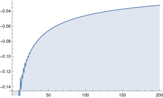
Here’s a plot to show the relative error in the approximation above.

Here’s the Mathematica code that made the plot.

    approx[n_] := Exp[Pi Sqrt[2 n/3]]/(4 n Sqrt[3])
    DiscretePlot[ 1 - approx[n]/PartitionsP[n], {n, 200}]

So the estimate above is always an under-estimate, at least about 4% low over the range we care about. It’s good enough for a quick calculation. It tells us, for example, to be very patient if we’re going to run any program that needs to iterate over all partitions of an integer even as small as 100.

The function PartitionsP above returns the number of partitions in its argument. It returned quickly, so it certainly did not generate all partitions and count them. Algorithms for computing p(n) might make an interesting blog post another time.

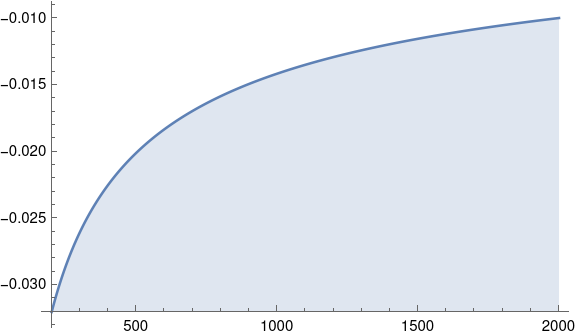
Even though it would be impractical to iterate over the partitions of larger values, we still might be curious what the plot above looks like for larger arguments. Let’s see what the plot would look like for n between 200 and 2000.

The shape of the curve is practically the same.

The relative error dropped by about a factor or 3 when we increased n by a factor of 10. So we’d expect if we increase n by another factor of 10, the relative error would drop about another factor of 3, and indeed that’s what happens: when n = 20,000, the relative error is about -0.003.

Vector spaces and subspaces over finite fields

Posted on 12 November 2021 by John

A surprising amount of linear algebra doesn’t depend on the field you’re working over. You can implicitly assume you’re working over the real numbers R and prove all the basic theorems—say all the theorems that come before getting into eigenvalues in a typical course—and all or nearly all of the theorems remain valid if you swap out the complex numbers for the real numbers. In fact, they hold for any field, even a finite field.

Subspaces over infinite fields

Given an n-dimensional vector space V over a field F we can ask how many subspaces of V there are with dimension k. If our field F is the reals and 0 < k < n then there are infinitely many such subspaces. For example, if n = 2, every line through the origin is a subspace of dimension 1.

Now if we’re still working over R but we pick a basis

e₁, e₂, e₃, …, e_n

and ask for how many subspaces of dimension k there are in V that use the same basis elements, now we have a finite number. In fact the number is the binomial coefficient

$\binom{n}{k}$

because there are as many subspaces as there are ways to select k basis elements from a set of n.

Subspaces over finite fields

Let F be a finite field with q elements; necessarily q is a prime power. Let V be an n-dimensional vector space over F. We might need to know how many subspaces of V there are of various dimensions when developing algebraic codes, error detection and correction codes based on vector spaces over finite fields.

Then the number of subspaces of V with dimension k equals the q-binomial coefficient

$\binom{n}{k}_q \equiv \frac{[n]_q!}{[k]_q! [n-k]_q!}$

mentioned in the previous post. Here [n]_q! is the q-factorial of n, defined by

$[n]_q! \equiv [1]_q [2]_q [3]_q \cdots [n]_q$

and [n]_q! is the q-analog of n, defined by

$[n]_q \equiv \frac{1 - q^n}{1-q} = 1 + q + q^2 + \cdots q^{n-1}$

The fraction definition holds for all n, integer or not, when q ≠ 1. The fraction equals the polynomial in q when n is a non-negative integer.

You can derive the expression for the number of subspaces directly from a combinatorial argument, not using any of the q-analog notation, but this notation makes things much more succinct.

Python code

We can easily code up the definitions above in Python.

    def analog(n, q):
        return (1 - q**n)//(1 - q)

    def qfactorial(n, q):
        p = 1
        for k in range(1, n+1):
            p *= analog(k, q)
        return p

    def qbinomial(n, k, q):
        d = qfactorial(k, q)*qfactorial(n-k, q)
        return qfactorial(n, q)/d

Example

To keep things small, let’s look at the field with q = 3 elements. Here addition and multiplication are carried out mod 3.

Let n = 3 and k = 1. So we’re looking for one-dimensional subspaces of F³ where F is the field of integers mod 3.

A one-dimensional subspace of vector space consists of all scalar multiples of a vector. We can only multiply a vector by 0, 1, or 2. Multiplying by 0 gives the zero vector, multiplying by 1 leaves the vector the same, and multiplying by 2 turns 1s into 2s and vice versa. So, for example, the vector (1, 2, 0) is a basis for the subspace consisting of

(0, 0, 0), (1, 2, 0}, (2, 1, 0).

We can find all the subspaces by finding a base for each subspace. And with a little brute force effort, here’s a list.

(1, 0, 0)
(0, 1, 0)
(0, 0, 1)
(0, 1, 1)
(1, 0, 1)
(1, 1, 0)
(1, 2, 0)
(0, 1, 2)
(2, 0, 1)
(1, 1, 1)
(2, 1, 1)
(1, 2, 1)
(1, 1, 2)

It’s easy to check that none of these vectors is a multiple mod 3 of another vector on the list. The theory above says we should expect to find 13 subspaces, and we have, so we must have found them all.

Mathematical plot twist: q-binomial coefficients

Posted on 12 November 2021 by John

The simplest instance of a q-analog in math is to replace a positive integer n by a polynomial in q that converges to n as q → 1. Specifically, we associate with n the polynomial

[n]_q = 1 + q + q² + q³ + … + q^n-1.

which obviously converges to n when q → 1.

More generally we can associate with a real number a the rational polynomial

[a]_q = (1 – q^a) / (1 – q).

When a is a positive integer, the two definitions are the same. When a is not an integer, you can see by L’Hôpital’s rule that

lim_{q → 1} [a]_q = a.

Motivation

Why would you do this? I believe the motivation was to be able to define a limit of a series where the most direct approach fails or is difficult to work with. Move over to the land of q-analogs, do all your manipulations there where requiring |q| < 1 avoids problems with convergence, then take the limit as q goes to 1 when you’re done.

q-factorials and q-binomial coefficients

The factorial of a positive integer is

n! = 1 × 2 × 3 × … × n

The q-factorial of n replaces each term in the definition of factorial with its q-analog:

[n]_q! = [1]_q [2]_q [3]_q … [n]_q

(It helps to think of []_q! as a single operator defining the q-factorial as above. This is not the factorial of [n]_q.)

Similarly, you can start with the definition of a binomial coefficient

n! / (k! (n–k)!)

and define the q-binomial coefficient by replacing factorials with q-factorials.

[n]_q! / ([k]_q! [n–k]_q!)

You can apply the same process to rising and falling powers, and then replace the rising powers in the definition of a hypergeometric function to define q-analogs of these functions.

(The q-analogs of hypergeometric functions are confusingly called “basic hypergeometric functions.” They are not basic in the sense of simple examples; they’re not examples at all but new functions. And they’re not basic in the sense of a basis in linear algebra. Instead, the name comes from q being the base of an exponent.)

Plot twist

And now for the plot twist promised in the title.

I said above that the q-analogs were motivated by subtle problems with convergence. There’s the idea in the background that eventually someone is going to let q approach 1 in a limit. But what if they don’t?

The theorems proved about q-analogs were first developed with the implicit assumption that |q| < 1, but at some point someone realized that the theorems don’t actually require this, and are generally true for any q. (Maybe you have to avoid q = 1 to not divide by 0 or something like that.)

Someone observed that q-analog theorems are useful when q is a prime power. I wonder who first thought of this and why. It could have been inspired by the notation, since q often denotes a prime power in the context of number theory. It could have been as simple as a sort of mathematical pun. What if I take the symbol q in this context and interpret it the way q is interpreted in another context?

Now suppose we have a finite field F with q elements; a theorem says q has to be a prime power. Form an n-dimensional vector space over F. How many subspaces of dimension k are there in this vector space? The answer is the q-binomial coefficient of n and k. I explore this further in the next post.

Another pentagonal number theorem

Posted on 11 November 2021 by John

An earlier post presented Euler’s pentagonal number theorem. This post presents a similar theorem by N. J. Fine developed two centuries later.

Define the jth pentagonal number by

P_j = j(3j – 1) / 2

where j can be any integer, e.g. j can be negative.

Theme

Let D_e(n) is the number of distinct partitions of n of even length and D_o(n) is the number distinct partitions of odd length. (See this post if any of these terms are unfamiliar.)

Euler’s pentagonal number theorem says

$D_e(n) - D_o(n) = \left\{ \begin{array}{ll} (-1)^j & \mbox{if } n = P_j \\ 0 & \mbox{otherwise} \end{array} \right.$

Variation

Euler discovered his theorem in 1741 and proved it a few years later. N. J. Fine published [1] the following variation on Euler’s theorem in 1948.

Define π_e(n) to be the number of partitions of n into distinct numbers, the largest of which is even, and define π_o(n) to be the number of partitions of n into distinct numbers, the largest of which is odd. Then Fine’s theorem says

$\pi_e(n) - \pi_o(n) = \left\{ \begin{array}{ll} -1 & \mbox{if } n = P_j \mbox{ for } j > 0 \\ \phantom{-}1 & \mbox{if } n = P_j \mbox{ for } j < 0 \\ \phantom{-}0 & \mbox{otherwise} \end{array} \right.$

Note that Euler and Fine have different ways of defining parity, the length of a partition versus the parity of the largest element. So, for example,

{8, 3, 2}

would count as an odd partition of 13 for Euler’s theorem, because it has length 3, but an even partition for Fine’s theorem, because the largest element is 8.

Both produce ±1 for pentagonal numbers and 0 otherwise. But the sign in Euler’s theorem depends on the parity of the index j. The parity in Fine’s theorem depends on the sign of j.

Mathematica

As in the previous two posts, we will illustrate the theorem here with Mathematica.

    distinctPartitionQ[list_] := Length[list] == Length[Union[list]]

    check[n_] := 
        Total[Map[(-1)^Max[#] &, 
              Select[IntegerPartitions[n], distinctPartitionQ]]] 

    Table[{n, check[n]}, {n, 1, 8}]

This returns

    {{1, -1}, {2, 1}, {3, 0}, {4, 0}, 
     {5, -1}, {6, 0}, {7, 1}, {8, 0}}

We get -1 for n = 1 = P₁ and for n = 5 = P₂.

We get 1 for n = 2 = P_-1 and for n = 7 = P_-2.

We get 0 for all other inputs because they are not pentagonal numbers.

[1] I found this in “Euler’s Pentagonal Number Theorem” by George E. Andrews, Mathematics Magazine, Vol. 56, No. 5 (Nov., 1983), pp. 279-284. Andrews cites “Some new results on partitions” by N. J. Fine, Proc. Nat. Acad. Sci. U.S.A., 34 (1948) 616-618.

Odd parts and distinct parts

Posted on 11 November 2021 by John

The previous post looked at a result of Euler regarding even and odd distinct partitions. This post will illustrate a related theorem by Euler.

Definitions

A partition of a positive integer n is a way of writing n as the sum of positive integers, without distinguishing the order of the terms, only the multi-set of summands.

For example, 6 can be written as

1 + 2 + 3

or as

3 + 2 + 1,

but these count as the same partition. Another possible partition of 6 is

3 + 1 + 1 + 1.

Here the summands form a multistet

{3, 1, 1, 1}.

This is not a set because the 1’s appear more than once. If the multiset of summands is actually a set, the partition is called a distinct partition.

A partition is called odd if every element is odd, and even if every element is even.

Theorem

Now we can state Euler’s theorem: The number of odd partitions of an integer equals the number of distinct partitions.

As before we will illustrate this with Mathematica.

Mathematica

First we define a couple predicate functions.

    distinctPartitionQ[list_] := Length[list] == Length[Union[list]]
    oddPartitionQ[list_] := And @@ Map[OddQ, list]

There are six odd partitions of 8:

    In: Select[IntegerPartitions[8], oddPartitionQ]
    Out: {{7, 1}, {5, 3}, {5, 1, 1, 1}, {3, 3, 1, 1}, 
          {3, 1, 1, 1, 1, 1}, {1, 1, 1, 1, 1, 1, 1, 1}}

And six distinct partitions of 8:

    In: Select[IntegerPartitions[8], distinctPartitionQ]
    Out: {{8}, {7, 1}, {6, 2}, {5, 3}, {5, 2, 1}, {4, 3, 1}}

To try partitions of more numbers, let’s define

    d[n_] := Length[Select[IntegerPartitions[n], distinctPartitionQ]] - 
             Length[Select[IntegerPartitions[n], oddPartitionQ]]

We can see that d[n] is 0 for n = 1, 2, 3, …, 50 by running

    Table[d[n], {n, 1, 50}]

Testing understanding

This post and the previous post illustrate something important: it helps to verify a theorem computationally, even if you know the theorem is true, in order to test your understanding of the theorem. If a theorem by Euler were wrong, we’d know by now. But my interpretation of the terms in this theorem and the theorem in the previous post were both wrong at first, and computations made this obvious.

Note that in this post, “odd partition” means a partition consisting of only odd numbers.

In the previous post, an “odd distinct partition” is a distinct partition of odd length. If we defined “odd distinct partition” to be a distinct partition consisting of only odd numbers, the statement of Euler’s pentagonal number theorem would be false.

For example, consider the distinct partitions of 3: 3 and 2+1. One distinct partition of even length and one of odd length, as the pentagonal number theorem predicts. But of these two partitions, one consists entirely of odd numbers, and none consists entirely of even numbers.

Partitions and Pentagons

Posted on 10 November 2021 by John

This post will present a remarkable theorem of Euler which makes a connection between integer partitions and pentagons.

Partitions

A partition of an integer n is a way of writing n as a sum of positive integers. For example, there are seven unordered partitions of 5:

5
4 + 1
3 + 2
3 + 1 + 1
2 + 2 + 1
2 + 1 + 1 + 1
1 + 1 + 1 + 1 + 1

Note that order does not matter. For instance, 4 + 1 and 1 + 4 count as the same partition. You can get a list of partitions of n in Mathematica with the function IntegerPartitions[n]. If we enter IntegerPartitions[5] we get

     {{5}, {4, 1}, {3, 2}, {3, 1, 1}, {2, 2, 1}, 
      {2, 1, 1, 1}, {1, 1, 1, 1, 1}}

We say a partition is distinct if all the numbers in the sum are distinct. For example, these partitions of 5 are distinct

5
4 + 1
3 + 2

but these are not

3 + 1 + 1
2 + 2 + 1
2 + 1 + 1 + 1
1 + 1 + 1 + 1 + 1

because each has a repeated number.

We can divide distinct partitions into those having an even number of terms and those having an odd number of terms. In the example above, there is one odd partition, just 5, and two even partitions: 4 + 1 and 3 + 2.

Pentagonal numbers

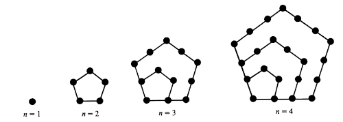
The pentagonal numbers are defined by counting the number of dots in a graph of concentric pentagons: 1, 5, 12, 22, …. This is OEIS sequence A000326.

The jth pentagonal number is

P_j = j(3j – 1) / 2.

We can define negative pentagonal numbers by plugging negative values of j into the equation above, though these numbers don’t have the same geometric interpretation. (I think they do have a geometric interpretation, but I forget what it is.)

Euler’s pentagonal number theorem

Leonard Euler discovered that the number of even distinct partitions of n equals the number of odd distinct partitions, unless n is a pentagonal number (including negative indices). If n is the jth pentagonal number, then the difference between the number of even and odd distinct partitions of n equals (-1)^j. In symbols,

$D_e(n) - D_o(n) = \left\{ \begin{array}{ll} (-1)^j & \mbox{if } n = P_j \\ 0 & \mbox{otherwise} \end{array} \right.$

Here D_e is the number of even distinct partitions and D_o is the number of odd distinct partitions.

Euler discovered this by playing around with power series and noticing that the series involved were generating functions for pentagonal numbers. Jordan Bell has written a commentary on Euler’s work and posted it on arXiv.

Mathematica examples

Let’s look at the partitions of 12, the 3rd pentagonal number.

IntegerPartions[12] shows there are 77 partitions of 12. We can pick out just the partitions into distinct numbers by selecting partition sets that have no repeated terms, i.e. that have as many elements as their union.

    Select[IntegerPartitions[12], Length[Union[#]] == Length[#] &]

This returns a list of 15 partitions:

    {{12},      {11, 1},   {10, 2},      {9, 3},    {9, 2, 1}, 
     {8, 4},    {8, 3, 1}, {7, 5},       {7, 4, 1}, {7, 3, 2}, 
     {6, 5, 1}, {6, 4, 2}, {6, 3, 2, 1}, {5, 4, 3}, {5, 4, 2, 1}}

Of these sets, 7 have an even number of elements and 8 have an odd number of elements. This matches what Euler said we would get because

7 – 8 = (-1)³.

We’d like to eplore this further without having to count partitions by hand, so let’s define a helper function.

    f[list_] := Module[
        {n = Length[Union[list]]}, 
        If [n == Length[list], (-1)^n, 0]
    ]

This function returns 0 for lists that have repeated elements. For sets with no repeated elements, it returns 1 for sets with an even number of elements and -1 for sets with an odd number of elements. If we apply this function to the list of partitions of n and take the sum, we get

D_e(n) – D_o(n).

Now

    Total[Map[f, IntegerPartitions[12]]]

returns -1. And we can verify that it returns (-1)^j for the jth pentagonal number. The code

    Table[Total[Map[f, IntegerPartitions[j (3 j - 1)/2]]], {j, -3, 3}]

returns

    {-1, 1, -1, 1, -1, 1, -1}

We can compute D_e(n) – D_o(n) for n = 1, 2, 3, …, 12 with

    Table[{n, Total[Map[f, IntegerPartitions[n]]]}, {n, 1, 12}]

and get

    {{1, -1}, {2, -1}, {3,  0}, {4,  0}, 
     {5,  1}, {6,  0}, {7,  1}, {8,  0}, 
     {9,  0}, {10, 0}, {11, 0}, {12, -1}}

which shows that we get 0 unless n is a pentagonal number.

Euler characteristic

Euler’s pentagonal number theorem reminds me of Euler characteristic. Maybe there’s a historical connection there, or maybe someone could formalize a connection even if Euler didn’t make the connection himself. In its most familiar form, the Euler characteristic of a polyhedron is

V – E + F

where V is the number of vertices, E is the number of edges, and F is the number of faces. Notice that this is an alternating sum counting o-dimensional things (vertices), 1-dimensional things (edges), and 2-dimensional things (faces). This is extended to higher dimensions, defining the Euler characteristic to be the alternating sum of dimensions of homology groups.

We can write D_e(n) – D_o(n) to make it look more like the Euler characteristic, using D_k(n) to denote the number of distinct partitions of size k.

D₀(n) – D₁(n) + D₂(n) – …

I suppose there’s some way to formulate Euler’s pentagonal number theorem in terms of homology.

Rising and falling powers

Posted on 9 November 2021 by John

I’ve mentioned rising powers several times recently. They come up in practice fairly often. Sometimes you see falling powers as well, and there’s a simple symmetry between the two.

There are multiple ways to denote rising powers, and lately I’ve used the Pochhammer notation (x)_k because it’s easy to type in HTML without having to inline any LaTeX. But it’s not the best notation. It’s not mnemonic, and it’s not completely standardized.

The notation in Concrete Mathematics is mnemonic, and symmetric between rising and falling powers. This book denotes rising powers by

$x^{\overline{k}} = x(x+1)(x+2) \cdots (x + k-1)$

and falling powers by

$x^{\underline{k}} = x(x-1)(x-2) \cdots (x - k + 1)$

The 0th rising and falling power of a number is defined to be 1 because empty products are conventionally defined to be 1.

Mathematica’s notation for rising and falling powers is not at all symmetric. The kth rising power of x is denoted

    Pochhammer[x, k]

and the kth falling power is denoted

    FactorialPower[x, k].

Falling powers came up a few days ago when I wrote about the tails of a gamma distribution. That post included the asymptotic series

$P(X > x) = \frac{x^{a-1}e^{-x}}{\Gamma(a)}\left( 1 + \frac{a-1}{x} + \frac{(a-1)(a-2)}{x^2} + \cdots\right)$

The series above could be written as

$\frac{x^{a-1} e^{-x}}{\Gamma(a)} \sum_{k=0}^\infty \frac{(a-1)^{\underline{k}}}{x^k}.$

Note that we used the fact that the 0th falling power of (a-1) is 1.

You can convert between rising and falling powers by

$\begin{align*} x^{\overline{k}} &= (-1)^k (-x)^{\underline{k}} \\ x^{\underline{k}} &= (-1)^k (-x)^{\overline{k}} \end{align*}$

Some resources will define rising powers but not falling powers or vice versa because the equations above make it easy to express everything in terms of just one or the other. In my experience, probability textbooks are likely to define falling powers but not rising powers, and books on special functions are likely to define rising powers but not falling powers.

Three kinds of confluence

Posted on 9 November 2021 by John

We say someone is fluent in a language if their words flow easily. The word fluent comes from the Latin fluere which means to flow. We say things are confluent if they flow together, such as the confluence of two streams.

This post will give three examples of the use of confluent in math and computer science:

confluent interpolation,
confluent functions, and
confluent reduction systems.

Confluent interpolation

Interpolation fills in the gaps between locations where a function’s values are known. If you’re given the values of a function f(x) at n+1 distinct points, there is a unique polynomial of degree n that takes on those values at those points.

Notice the above paragraph stipulated distinct points. If two of your point are actually different labels for the same point, your interpolation problem is either inconsistent and over-determined, or it is consistent but under-determined.

Suppose you have two points x₁ and x₂ that start out as distinct but move together. Once they become equal, information is lost. But if you kept track of the slope of the line joining f(x₁) and f(x₂) as the points moved together, in the limit you have the derivative f ′(x₁). The derivative restores information that otherwise would have been lost.

Confluent interpolation specifies the values of the function f(x) at distinct points. At doubled points, it specifies a consistent function value and the value of the derivative.

Incidentally, just as the Vandermonde matrix arises in ordinary interpolation, the confluent Vandermonde matrix arises in confluent interpolation.

Confluent functions

The previous post showed that the error function erf(x) is closely related to a special function known as a “confluent hypergeometric function.”

The hypergeometric differential equation has regular singular points at 0, 1, and ∞. If we take a limit that pushes the singularity at 1 off to ∞, we get Kummer’s differential equation, the equation satisfied by confluent hypergeometric functions.

Confluent reduction systems

A reduction system is said to be confluent if whenever a term x can be reduced in a finite number of steps to two different terms y₁ and y₂, there is a common term that both y₁ and y₂ can be reduced to. In symbols:

$y_1 \xleftarrow{*} x \xrightarrow{*} y_2 \implies y_1 \downarrow y_2$

The Church-Rosser theorem says that lambda calculus is confluent. If two ways of applying reduction rules to the same lambda expression terminate, they terminate in the same expression. Not all term rewriting systems are confluent, but lambda calculus is.

Three error function series

Posted on 7 November 2021 by John

A common technique for numerically evaluating functions is to use a power series for small arguments and an asymptotic series for large arguments. This might be refined by using a third approach, such as rational approximation, in the middle.

The error function erf(x) has alternating series on both ends: its power series and asymptotic series both are alternating series, and so both are examples that go along with the previous post.

The error function is also a hypergeometric function, so it’s also an example of other things I’ve written about recently, though with a small twist.

The error function is a minor variation on the normal distribution CDF Φ. Analysts prefer to work with erf(x) while statisticians prefer to work with Φ(x). See these notes for translating between the two.

Power series

The power series for the error function is

$\text{erf}(x) = \frac{2}{\sqrt{\pi}} \sum_{n=0}^\infty (-1)^n \frac{x^{2n+1}}{n!(2n+1)}$

The series converges for all x, but it is impractical for large x. For every x the alternating series theorem eventually applies, but for large x you may have to go far out in the series before this happens.

Asymptotic series

The complementary error function erfc(x) is given by

erfc(x) = 1 – erf(x).

Even though the relation between the two functions is trivial, it’s theoretically and numerically useful to have names for both functions. See this post on math functions that don’t seem necessary for more explanation.

The function erfc(x) has an alternating asymptotic series.

$\text{erfc}(x) = \frac{e^{-x^2}}{\sqrt{\pi}x} \sum_{n=0}^\infty (-1)^n\frac{(2n-1)!!}{2^n} x^{-2n}$

Here a!!, a double factorial, is the product of the positive integers less than or equal to a and of the same parity as a. Since in our case a = 2n – 1, a is odd and so we have the product of the positive odd integers up to and including 2n – 1. The first term in the series involves (-1)!! which is defined to be 1: there are no positive integers less than or equal to -1, so the double factorial of -1 is an empty product, and empty products are defined to be 1.

Confluent hypergeometric series

The error function is a hypergeometric function, but of a special kind. (As is often the case, it’s not literally a hypergeometric function but trivially related to a hypergeometric function.)

The term “hypergeometric function” is overloaded to mean two different things. The strictest use of the term is for functions F(a, b; c; x) where the parameters a and b specify terms in the numerator of coefficients and the parameter c specifies terms in the denominator. You can find full details here.

The more general use of the term hypergeometric function refers to functions that can have any number of numerator and denominator terms. Again, full details are here.

The special case of one numerator parameter and one denominator parameter is known as a confluent hypergeometric function. Why “confluent”? The name comes from the use of these functions in solving differential equations. Confluent hypergeometric functions correspond to a case in which two singularities of a differential equation merge, like the confluence of two rivers. More on hypergeometric functions and differential equations here.

Without further ado, here are two ways to relate the error function to confluent hypergeometric functions.

$\text{erf}(x) = \frac{2x}{\sqrt{\pi}} F\left(\frac{1}{2}; \frac{3}{2}; -x^2\right) = \frac{2x}{\sqrt{\pi}} e^{-x^2} F\left(1; \frac{3}{2}; x^2\right)$

The middle expression is the same as power series above. The third expression is new.

Solving hard problems

Lambert’s W function

Basic bootstrapping

Putting it all together

More Lambert W posts

Subspaces over infinite fields

Subspaces over finite fields

Python code

Example

Related posts

Motivation

q-factorials and q-binomial coefficients

Plot twist

Related posts

Theme

Variation

Mathematica

Related

Definitions

Theorem

Mathematica

Testing understanding

Partitions

Pentagonal numbers

Euler’s pentagonal number theorem

Mathematica examples

Euler characteristic

Confluent interpolation

Confluent functions

Confluent reduction systems

Related posts

Power series

Asymptotic series

Confluent hypergeometric series