Three error function series

A common technique for numerically evaluating functions is to use a power series for small arguments and an asymptotic series for large arguments. This might be refined by using a third approach, such as rational approximation, in the middle.

The error function erf(x) has alternating series on both ends: its power series and asymptotic series both are alternating series, and so both are examples that go along with the previous post.

The error function is also a hypergeometric function, so it’s also an example of other things I’ve written about recently, though with a small twist.

The error function is a minor variation on the normal distribution CDF Φ. Analysts prefer to work with erf(x) while statisticians prefer to work with Φ(x). See these notes for translating between the two.

Power series

The power series for the error function is

\text{erf}(x) = \frac{2}{\sqrt{\pi}} \sum_{n=0}^\infty (-1)^n \frac{x^{2n+1}}{n!(2n+1)}

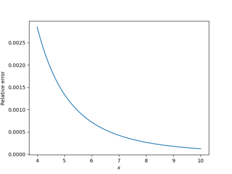
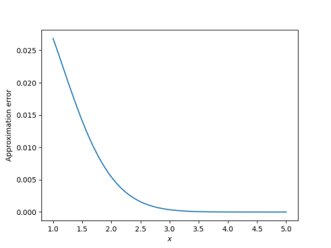
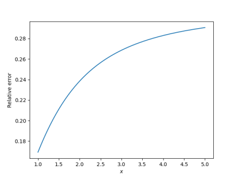
The series converges for all x, but it is impractical for large x. For every x the alternating series theorem eventually applies, but for large x you may have to go far out in the series before this happens.
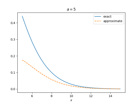
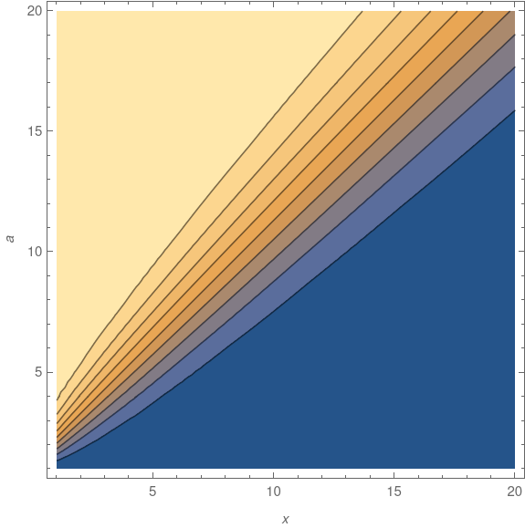
Asymptotic series

The complementary error function erfc(x) is given by

erfc(x) = 1 − erf(x).

Even though the relation between the two functions is trivial, it’s theoretically and numerically useful to have names for both functions. See this post on math functions that don’t seem necessary for more explanation.

The function erfc(x) has an alternating asymptotic series.

\text{erfc}(x) = \frac{e^{-x^2}}{\sqrt{\pi}x} \sum_{n=0}^\infty (-1)^n\frac{(2n-1)!!}{2^n} x^{-2n}

Here a!!, a double factorial, is the product of the positive integers less than or equal to a and of the same parity as a. Since in our case a = 2n − 1, a is odd and so we have the product of the positive odd integers up to and including 2n − 1. The first term in the series involves (−1)!! which is defined to be 1: there are no positive integers less than or equal to −1, so the double factorial of −1 is an empty product, and empty products are defined to be 1.

Confluent hypergeometric series

The error function is a hypergeometric function, but of a special kind. (As is often the case, it’s not literally a hypergeometric function but trivially related to a hypergeometric function.)

The term “hypergeometric function” is overloaded to mean two different things. The strictest use of the term is for functions F(a, b; c; x) where the parameters a and b specify terms in the numerator of coefficients and the parameter c specifies terms in the denominator. You can find full details here.

The more general use of the term hypergeometric function refers to functions that can have any number of numerator and denominator terms. Again, full details are here.

The special case of one numerator parameter and one denominator parameter is known as a confluent hypergeometric function. Why “confluent”? The name comes from the use of these functions in solving differential equations. Confluent hypergeometric functions correspond to a case in which two singularities of a differential equation merge, like the confluence of two rivers. More on hypergeometric functions and differential equations here.

Without further ado, here are two ways to relate the error function to confluent hypergeometric functions.

\text{erf}(x) = \frac{2x}{\sqrt{\pi}} F\left(\frac{1}{2}; \frac{3}{2}; -x^2\right) = \frac{2x}{\sqrt{\pi}} e^{-x^2} F\left(1; \frac{3}{2}; x^2\right)

The middle expression is the same as power series above. The third expression is new.

A more powerful alternating series theorem

In application you often truncate an infinite series to give a practical approximation. Ideally you’d like to know how accurate the approximation is. It would be even better to know the sign of the error of the approximation.

Alternating series let you do this. But some forms of the alternating series theorem leave money on the table. That is, a more general and more useful form of the theorem is possible.

Weak statement

Here’s a weak statement of the alternating series theorem taken from a textbook.

If a1a2a3 ≥ … ≥ an ≥ … 0 for all n, then the alternating series

a1a2 + a3a4 + …

converges to a real number S. Moreover, if the nth partial sums is denoted Sn then

|SSn| ≤ Sn+1.

The notation above is a little vague when it says “… 0”. The theorem requires that all the a‘s are non-negative and that their limit is 0.

Small improvements

One easy improvement is to note that it’s only necessary for the terms to eventually satisfy the conditions of the theorem. If the terms don’t initially decrease in absolute value, or don’t initially alternate in sign, then apply the theorem starting after a point where the terms do decrease in absolute value and alternate in sign.

Another improvement is to note that we can tell the sign of the truncation error. That is, if Sn+1 is positive, then

0 ≤ SSnSn+1,

and if Sn+1 is negative, then

Sn+1SSn ≤ 0.

Stronger statement

A stronger statement of the alternating series theorem is to note that it is not necessary for all the terms to alternate. Also, you can have truncation error estimates even if the series doesn’t converge.

Here is a much stronger statement of the alternating series theorem, taken from the book Interpolation by J. F. Steffensen, with notation changed to match the theorem above.

Let

S = a1 + a2 + … + an + Rn+1

and let the first non-zero term after an be an+s. If Rn+1 and Rn+s+1 have opposite signs then the remainder term is numerically smaller than the first rejected non-zero term, and has the same sign.

Note that there’s no issue of convergence, and so the theorem could be applied to a divergent series. And there’s no requirement that the terms alternate signs, only that the specified remainder terms alternate signs.

Applications

A lot of functions that come up in applications have alternating series representations. If a series does not alternate, it can be useful to look for a reformulation that does have an alternating series, because, as explained here, truncation error is easy to estimate. Alternating series can also often be accelerated.

The next post shows that the error function, a slight variation on the Gaussian cumulative distribution function, has both an alternating power series and an alternating asymptotic series.

Gamma distribution tail probability approximation

This post will approximate of the tail probability of a gamma random variable using the heuristic given in the previous post.

The gamma distribution

Start with the integral defining Γ(a). Divide the integrand by Γ(a) so that it integrates to 1. This makes the integrand into a probability density, and the resulting probability distribution is called the gamma distribution with shape a. To evaluate the probability of this distribution’s tail, we need to integrate

\frac{1}{\Gamma(a)} \int_x^\infty t^{a-1} \exp(-t)\, dt

This distribution has mean and variance a, and mode a − 1.

We’re interested in approximating the integral above for moderately large x relative to a.

Approximation

To apply the 1/e heuristic we need to find a value of t such that

ta−1 exp(−t) = xa−1 exp(−x)/e = xa−1 exp(− x − 1).

This equation would have to be solved numerically, but lets try something very simple first and see how it works. Let’s assume the ta−1 term doesn’t change as much as the the exp(−t) term between x and x + 1. This says an approximate solution to our equation for t is simply

t = x + 1

and so the base of our rectangle runs from x to x + 1, i.e. has width 1. So the area of our rectangle is simply its height. This gives us

\frac{1}{\Gamma(a)} \int_x^\infty t^{a-1} \exp(-t)\, dt \approx \frac{x^{a-1}\exp(-x)}{\Gamma(a)}

In other words, the CDF is approximately the PDF. That’s all nice and simple, but how good is it? Here’s a plot for a = 5.

So is this good or not? It’s not a question of whether but of which. It’s a poor approximation for some parameters but a very good approximation for others. The approximation improves when a is closer to 1 and when x is larger.

We were kinda sloppy in solving for t above. Would it help if we had a more accurate value of t? No, that doesn’t make much difference, and it actually makes things a little worse. The important issue is to identify over what range of a and x the approximation works well.

Asymptotic series

It turns out that our crude integration estimate happens to correspond to the first term in an asymptotic series for our integral. If X is a gamma random variable with shape a then we have the following asymptotic series for the tail probability.

P(X > x) = \frac{x^{a-1}e^{-x}}{\Gamma(a)}\left( 1 + \frac{a-1}{x} + \frac{(a-1)(a-2)}{x^2} + \cdots\right)

So if we truncate the portion inside the parentheses to just 1, we have the approximation above. The approximation error from truncating an asymptotic series is approximately the first term that was left out.

So if x is much larger than a, the approximation error is small. Since the expected value of X is a, the tail probabilities correspond to values of x larger than a anyway. But if x is only a little larger than a, the approximation above won’t be very good, and adding more terms in the series won’t help either.

Here’s a contour plot of the absolute error:

The deep blue area below the diagonal of the graph shows the error is smallest when x > a. In 3D, the plot has a high plateau in the top left and a valley in the lower right, with a rapid transition between the two, suggested by the density of contour lines near the diagonal.

Epilogue

In the previous post I said that the next post would give an example where the 1/e heuristic doesn’t work well. This post has done that. It’s also given an example when the heuristic works very well. Both are the same example but with different parameters. When x >> a the method works well, and the bigger x is relative to a, the better it works.


The 1/e heuristic

The previous post looked at the FWHM (full width at half maximum) technique for approximating integrals, applied to the normal distribution.

This post is analogous, looking at the 1/e heuristic for approximating integral. We will give an example in this post where the heuristic works well. The next post will give an example where the heuristic works poorly.

The 1/e heuristic

In a function decays roughly exponentially, one way to approximate its integral is by the area of a rectangle with height equal to the maximum value of the integrand, and with base extending to the point where the integrand decreases by a factor of e, i.e. where its value is 1/e times less than the initial value. This technique is discussed in the book Street-fighting Mathematics.

This technique gives the exact value when integrating exp(−x) from 0 to infinity, and so it seems reasonable that it would give a good approximation for integrals that behave something like exp(−x).

First example

For the first example we will look at the integral

\int_x^\infty exp\left(\frac{1}{t} - t \right) \, dt

for x > 0. We’re especially interested in large x.

To find where the integrand has dropped by a factor of e we need to solve

exp(1/t − t) = exp(1/xx − 1)

for fixed x. Taking logs shows we need to solve

t² − at − 1 = 0

where

ax + 1/xx + 1.

Applying the quadratic formula and taking the positive solution gives

t = \frac{a +\sqrt{a^2 + 4}}{2} \approx a + \frac{1}{a}

We approximate our integral by the area of a rectangle with height

exp(x + 1/x)

and width

(a + 1/a) − x.

The plot below show that not only is the absolute error small, as one would expect, the relative error is small as well and decreases rapidly as x increases.

Simple normal distribution tail estimate

A very common task in probability and statistics is to estimate the probability of a normal random variable taking on a value larger than a given value x. By shifting and scaling we can assume our normal random variable has mean 0 and variance 1. This means we need to approximate the integral

 \frac{1}{\sqrt{2\pi}}\int_x^\infty \exp(-t^2/2)\, dt

We are interested in positive values of x, especially moderately large values of x.

We will estimate the integral above using the FWHM trick. This technique approximates the area under a curve by the area of a single rectangle.

The height of the rectangle is the maximum value of the integrand. The width is the distance between two points where the integrand takes on half its maximum value. The FWHM technique takes its name from the base of this rectangle: Full Width between points of Half Maximum.

In our example, the integrand is strictly decreasing over the region of integration. This means the maximum occurs at the beginning, at x, and there’s only one place where the integrand takes on half its maximum value. So the base of our rectangle runs from x to the point t where the integrand drops by a half.

To find t we need to solve

 \exp(-t^2/2) = \exp(-x^2/2)/2

to get

t = \sqrt{x^2 + 2 \log 2}

It follows that

\frac{1}{\sqrt{2\pi}}\int_x^\infty \exp(-t^2/2)\, dt \approx \frac{1}{\sqrt{2\pi}} \left(\sqrt{x^2 + 2 \log 2} - x\right) \exp(-x^2/2)

Note that the base of our rectangle, tx, is on the order of 1/x, and so the estimate above is roughly similar to the rigorous bounds on normal tail probabilities given here.

So how good is the approximation? We can compute the error with the following Python code.

    import numpy as np
    import matplotlib.pyplot as plt
    from scipy.stats import norm

    x = np.linspace(1, 5, 100)
    approx = (2*np.pi)**-0.5 * np.exp(-x**2/2)
    approx *= ((x*x + 2*np.log(2))**0.5 - x)
    error = exact - approx

Here’s a plot of the error:

So the approximation error is small, and gets smaller as x increases. Depending on context, the error may be small enough.

However, Gaussian tail probabilities decrease rapidly, so we should ask whether the approximation error is small relative to the exact value. So we plot

    relative = error/exact

Here the results are not as impressive.

The relative error is on the order of 20%, and it actually increases as x increases. This tells us our approximation is not an asymptotic approximation. Still, it’s not bad for such a crude derivation.

Related posts

Marden’s amazing theorem

The previous post was a warmup for this post. It gave an example of the theorem that if p is a polynomial, the roots of its derivative p′ lie inside the convex hull of the roots of p. If p is a cubic polynomial, we can say much more.

Suppose p(z) is a polynomial with three distinct roots, not all on a line. Then the roots of p are the vertices of a triangle T in the complex plane. We know that the roots of p′ lie inside T, but Marden’s theorem says where they lie inside T.

Let E be the unique ellipse inscribed inside T that touches T at the midpoint of each side. Then Marden’s theorem says that the roots of p′ lie on the foci of E.

The ellipse E is sometimes called the Steiner inellipse.

For an example, let

p(z) = z (z − 3) ( − 2 − 4i)

The roots of the derivative of p are 1.4495 + 0.3100i and 1.8838 + 2.3566i.

Here’s a plot of the roots of p (blue dots), the roots of p′ (orange ×), and the Steiner ellipse. I used a parametric equation for the Steiner ellipse from here.

Related posts

Convex hull of zeros

There’s a well-known theorem in complex analysis that says that if p is a polynomial, then the zeros of its derivative p′ lie inside the convex hull of the zeros of p. The convex hull of a set of points is the smallest convex set containing those points.

This post gives a brief illustration of the theorem. I created a polynomial with roots at 0, i, 2 + i, 3-i, and 1.5+0.5i. The convex hull of these points is the quadrilateral with corners at the first four roots; the fifth root is inside the convex hull of the other roots.

The roots are plotted with blue dots. The roots of the derivative are plotted with orange ×’s.

In the special case of cubic polynomials, we can say a lot more about where the roots of the derivative lie. That is the topic of the next post.

More complex analysis posts

Escaping the unit disk

Hypergeometric functions are defined in terms of their power series representation. This power series converges inside the unit circle and diverges outside. The functions extend to most [1] of the complex plane, and do so in a computationally nice way.

Analytic continuation is often sort of existential: we prove that it can be done, but we may not be able to say much explicitly about the result. But for hypergeometric functions, there is an explicit formula.

This formula is so complicated that it’s possible to miss its basic structure. Here’s an outline version:

F(\ldots z) = \ldots F(\ldots z^{-1}) + \ldots F(\ldots z^{-1})

This says that F evaluated at a point z outside of the unit circle is equal to the sum of two terms involving F evaluated at 1/z, a point inside the unit circle. This means you can evaluate F everywhere [1] if you can evaluate it inside the unit circle.

The parameters in each of the F‘s above are different, so the formula doesn’t relate a single function’s value at z to the same function’s values at 1/z. Instead, it relates the value of one instance of a class of functions at z to values of other instances of the class at 1/z.

And now without further ado, here is the analytic continuation formula in all its glory:

\begin{align*}  \frac{\Gamma(a)\Gamma(b)}{\Gamma(c)}F(a, b;c; z) &=  \frac{\Gamma(a)\Gamma(b-a)}{\Gamma(c-a)} \,\,(-z)^{-a}\,\,F(a, 1-c+a; 1-b+a; z^{-1}) \\ &+ \,\frac{\Gamma(b)\Gamma(a-b)}{\Gamma(c-b)} \,\,(-z)^{-b}\,\,F(b,\, 1-c+b; 1-a+b; z^{-1}) \end{align*}

[1] There may be a singularity at 1, and there may be a branch cut along the real axis from 1 to infinity.

Raabe’s convergence test

The ratio test for the convergence of a series is inconclusive if the ratio of consecutive terms converges to 1. There are more advanced variations on the ratio test, such as Raabe’s test than may succeed when the basic ratio test fails.

For example, consider the hypergeometric function F(11, 3; 21; z) with parameters taken from today’s date: 11/3/21. Since hypergeometric functions are symmetric in their first two parameters, European readers are welcome to think of this function as F(3, 11; 21; z).

F(11, 3; 21; z) = 1 + \frac{11\cdot 3}{21\cdot 1}z + \frac{11\cdot 12 \cdot 3\cdot 4}{21\cdot 22\cdot 1\cdot 2}z^2 + \cdots

The coefficient of zk is

(11)k (3)k / (21)k (1)k

where

(a)k = a (a+1) (a + 2) … (a + k – 1)

is the kth rising power of a.

The series defining F(11, 3; 21; z) converges uniformly if |z| < 1 and diverges if |z| > 1. What happens on the unit circle where |z| = 1?

The ratio of the absolute value of consecutive terms is

\frac{a_n}{a_{n+1}} = \frac{(n+21)(n+1)}{(n+11)(n+3)} = 1 + \frac{8}{n} - {\cal O}\left(\frac{1}{n^2} \right)

which converges to 1 as n → ∞. The basic ratio test is inconclusive.

Raabe’s ratio test says to consider

\rho_n = n\left(\frac{a_n}{a_{n+1}} - 1 \right)

If the limit (more generally the lim inf) of ρn is greater than 1, the series converges. if the limit (more generally the lim sup) of ρn is less than 1, the series diverges.

In our case the limit of ρn is 8, and so F(11, 3; 21; z) converges everywhere on the unit circle.

Like the basic ratio test, Raabe’s test may also be inconclusive. In that case there are more powerful tests to try, such as Kummer’s test, though it and all related tests may turn out inconclusive.

By the way Mr. Raabe’s name came up here a couple weeks ago in the context of Bernoulli polynomials.

Hypergeometric equation

I’ve asserted numerous times here that hypergeometric functions come up very often in applied math, but I haven’t said why. This post will give one reason why.

One way to classify functions is in terms of the differential equations they satisfy. Elementary functions satisfy simple differential equations. For example, the exponential function satisfies

y′ = y

and sine and cosine satisfy

y″ + y = 0.

Second order linear differential equations are common and important because Newton’s are second order linear differential equations. For the rest of the post, differential equations will be assumed to be second order and linear, with coefficients that are analytic except possibly at isolated singularities.

ODEs can be classified in terms of the sigularities of their coefficients. The equations above have no singularities and so their solutions are some of the most fundamental equations.

If an ODE has two or fewer regular singular points [1], it can be solved in terms of elementary functions. The next step in complexity is to consider differential equations whose coefficients have three regular singular points. Here’s the kicker:

Every ODE with three regular singular points can be transformed into the hypergeometric ODE.

So one way to think of the hypergeometric differential equation is that it is the standard ODE with three regular singular points. These singularities are at 0, 1, and ∞. If a differential equation has singularities elsewhere, a change of variables can move the singularities to these locations.

The hypergeometric differential equation is

x(x − 1) y″ + (c − (a + b + 1)x) y′ + ab y = 0.

The hypergeometric function F(a, b; c; x) satisfies this equation, and if c is not an integer, then a second independent solution to the equation is

x1−c F(1 + ac, 1 + bc; 2 − c; x).

To learn more about the topic of this post, see Second Order Differential Equations: Special Functions and Their Classification by Gerhard Kristensson.

Related posts

[1] This includes singular points at infinity. A differential equation is said to have a singularity at infinity if under the change of variables t = 1/x the equation in u has a singularity at 0. For example, Airy’s equation

y″ + x y = 0

has no singularities in the finite complex plane, and it has no solution in terms of elementary functions. This does not contradict the statement above because the equation has a singularity at infinity.