An interesting recursion

The previous post concerned finding the inverse of a function with respect to Dirichlet convolution. Given a function f defined on the positive integers, we want to find a function g, also defined on positive integers, such that f*g = δ. This means we want to find a function g such that the sum

(f*g)(n) = \sum_{d|n} f(d) \,\,g\left(\frac{n}{d} \right)

evaluates to 1 if n = 1 and 0 otherwise.

We said in that post that the function g can be defined recursively by

g(1) =\frac{1}{f(1)}

and

g(n) = -\frac{1}{f(1)} \sum_{\stackrel{d > 1}{d|n}} f(d)\,\,g\left(\frac{n}{d} \right )

for n > 1.

Python code

We can implement this directly in Python as a recursive function. Starting with any function f, we can define g exactly as above. For simplicity we set f(n) = n in the code below.

    from sympy import divisors

    def f(n):
        return n

    def g(n):
        if n == 1:
            return 1/f(1)
        s = sum(f(d)*g(n//d) for d in divisors(n)[1:])
        return -s/f(1)

The function sympy.divisors returns a list of divisors of a number, sorted in increasing order. We use [1:] to exclude the 0th divisor, i.e. 1, to get the list of divisors greater than 1. The code terminates because d > 1, and so n/d < n.

Note that the code uses integer division in g(n//d). Since we’re dividing n by one of its divisors, n/d is (mathematically) an integer, but the Python code n/d would return a value of type float and cause Python to complain that an argument to g is not an integer.

What’s interesting about this recursion is the set of cases g is defined by. Often a recursive function of n is defined in terms of its value at n-1, as in factorial, or its values at consecutive previous values, as in Fibonacci numbers. But here the value of g at n depends on the the values of g at factors of n.

So, for example, if we evaluate g(12), the code will evaluate g at 1, 2, 3, 4, and 6. In the process of computing g(12) we don’t need to know the value of g at 11.

Caching

Note that there’s some redundancy in the execution of our code. When we evaluate g at 4, for example, it evaluates g at 2, which had already been calculated. We could eliminate this redundancy by using memoization to cache computed values. In Python this can be done with the lru_cache decorator from functools.

    import functools

    @functools.lru_cache(maxsize=None)
    def g(n):
        if n == 1:
            return 1/f(1)
        s = sum(f(d)*g(n//d) for d in divisors(n)[1:])
        return -s/f(1)

If we use the revised code to calculate g(12), the call to g(6), for example, will look up the previously computed values of g(1), g(2), and g(3) from a cache.

If we evaluate g at several values, the code will fill in its cache in a scattered sort of way. If our first call is to evaluate g(12), then after that call the values of g at 1, 2, 3, 4, and 6 will be cached, but there will be no value of g at 7, for example, in the cache. If we then evaluate g(7), then this value will be cached, but there’s no value of g at 5 in the cache, and there won’t be until after we evaluate g at a multiple of 5.

Run time

Suppose the cache contains g(x) for all x < n and you want to compute g(n). How long would that take?

For large n, the number of divisors of n is on average about log(n), so the algorithm requires O(log n) look ups. For more detail, see the Dirichlet divisor problem. If you wanted to be more detailed in your accounting, you’d need to take into account the time required to produce the list of n‘s divisors, and the time required to look up cached values. But as a first approximation, the algorithm runs in O(log n) time.

I think the same is true even if you start with an empty cache. It would take longer in this case, but I think this would only change the size of the constant in front of log n.

Related posts

Dirichlet convolution

That can’t be right

I was skimming a book on number theory [1] recently and came across the following theorem that makes no sense out of context:

An arithmetical function f has an inverse if and only if f(1) ≠ 0.

Wait, what?! That’s obviously false unless I’ve missed something. Maybe “arithmetical function” is far more restrictive than I thought.

No, in this book an arithmetical function is simply a function on positive integers. In general it can be complex-valued, though early in the book all the examples are integer or rational valued.

What I was missing was the meaning of “inverse.” My first thought was that it meant inverse with respect to composition, but it meant inverse with respect to convolution.

Dirichlet convolution

Given two arithmetic functions f and g, their Dirichlet convolution f*g is defined by

(f*g)(n) = \sum_{d|n} f(d) \,\,g\left(\frac{n}{d} \right)

The sum is over all divisors of n and so, for example, the value of f * g at 6 would be

f(1)g(6) + f(2)g(3) + f(3)g(2) + f(6)g(1)

It’s clear that convolution is commutative, and with a little more effort you can show that it’s associative.

There is an identity element for convolution, the function δ(n) defined to be 1 if n = 1 and 0 otherwise. For any arithmetical function f, clearly f*δ = f because all the terms in the sum defining (f*δ)(n) are zero except the term f(n).

Inverse

In the context of the theorem above, the inverse of a function f is another function g whose convolution with f gives the identity δ, i.e. g is the inverse of f if f*g = δ. Inverses, if they exist, are unique.

Now that we have the right definition of inverse in mind, the theorem above isn’t obviously false, but it’s not clear why it should be true. And it’s a remarkable statement: with just the slightest restriction, i.e. f(1) ≠ 0, every arithmetical function has an inverse with respect to convolution. Not only that, the proof is constructive, so it shows how to compute the inverse.

For an arithmetical function f with f(1) ≠ 0, define its inverse function g by

g(1) =\frac{1}{f(1)}

and for n > 1 define

g(n) = -\frac{1}{f(1)} \sum_{\stackrel{d > 1}{d|n}} f(d)\,\,g\left(\frac{n}{d} \right )

This definition is not circular even though g appears on both sides. On the right side g is only evaluated at arguments less than n since the sum restricts d to be greater than 1. The next post implements this recursive definition of g in Python.

Möbius inversion formula

Define the function ζ to be the constant function 1. Since ζ(1) is not zero, ζ has an inverse. Call that inverse μ.

If f = g*ζ, then convolution of both sides with μ shows that f*μ = g. This is the Möbius inversion formula.

When presented this way, the Möbius inversion formula looks trivial. That’s because all the hard work has been moved into prerequisites. Stated from scratch, the theorem is more impressive. Without using any of the definitions above, Möbius inversion formula says that if f is defined by

f(n) = \sum_{d|n}g(d)

then

g(n) = \sum_{d|n}f(d) \, \mu\left(\frac{n}{d} \right)

where

\mu(n) = \left\{ \begin{aligned} {1} &\mbox{\quad if } {n=1} \\ {0} &\mbox{\quad if } {a^2 \,|\, n \mbox{ for some } a > 1} \\ {(-1)^r} &\mbox{\quad if } {n \mbox{ has } r \mbox{ distinct prime factors}} \end{aligned} \right.

We initially defined μ implicitly as the inverse of the constant function 1. When written out explicitly we have the definition of the Möbius function μ above.

Related posts

[1] An Introduction of Arithmetical Functions by Paul J. McCarthy, Springer-Verlag, 1986.

Nota bene

NB

I was looking at the J programming language yesterday and I was amused to see that it uses “NB.” to mark the rest of a line of source code as a comment, just like # in Python or // in C++. This makes comments in J look like comments in English prose.

“NB” abbreviates the Latin phrase nota bene meaning “note well.” It’s been used to mark side notes in English for about three centuries.

Most programming languages couldn’t use “NB” or “NB.” as a comment marker because it would inconsistent with conventions for identifiers, but J’s unconventional code syntax allows it to use conventional English notation for comments.

Why J?

I was looking at J because I have a project looking at its younger sister Remora. As described in this paper,

Remora is a higher-order, rank-polymorphic array-processing programming language, in the same general class of languages as APL and J. It is intended for writing programs to be executed on parallel hardware.

J keeps the array-oriented core of APL but drops its infamous symbols. Remora syntax is even closer to the mainstream, being written like a Lisp. (Some might object that Lisp isn’t mainstream, but it sure is compared to APL or J.)

APL comment symbol

Learning about J’s comment marker made me curious what its APL counterpart was. APL had custom symbols for everything, including comments. Comments began with ⍝ (U+235D), the idea being that the symbol looked like a lamp, giving light to the poor soul mentally parsing code.

U+235D APL FUNCTIONAL SYMBOL UP SHOE JOT

The full name for the lamp symbol is “APL FUNCTIONAL SYMBOL UP SHOE JOT.” Since this section of code is explicitly for APL symbols, why not call the symbol  COMMENT or LAMP rather than UP SHOE JOT?

I suppose the comment symbol looks like the bottom of a shoe. There’s also a symbol ⍦ (U+2366) [1] with the name “APL FUNCTIONAL SYMBOL DOWN SHOE STILE”

APL FUNCTIONAL SYMBOL DOWN SHOE STILE

and so “up” and “down” must refer to the orientation of the part of the symbol that looks like ∩ and ∪. But what about “jot” and “stile”?

A jot is a small character. The name is related to the Greek letter iota (ι) and the Hebrew letter yod (י). But if ∩ and ∪ are a shoe, the “jot” is a fairly large circle. Does “jot” have some other meaning?

A “stile” is a step or a rung, as in a turnstile. I suppose the vertical bar on top of ∪ is a stile.

Related posts

[1] What is this character for in APL? Unicode includes it as an APL symbol, but it’s not included in Wikipedia’s list of APL symbols.

What’s “differential” about differential privacy?

Interest in differential privacy is growing rapidly. As evidence of this, here’s the result of a Google Ngram search [1] on “differential privacy.”

Graph rapidly rising from 2000 to 2019

When I first mentioned differential privacy to consulting leads a few years ago, not many had heard of it. Now most are familiar with the term, though they may not be clear on what it means.

The term “differential privacy” is kinda mysterious, particularly the “differential” part. Are you taking the derivative of some privacy function?!

In math and statistics, the adjective “differential” usually has something to do with calculus. Differential geometry applies calculus to geometry problems. Differential equations are equations involving the derivatives of the function you’re after.

But differential privacy is different. There is a connection to differential calculus, but it’s further up the etymological tree. Derivatives are limits of difference quotients, and that’s the connection. Differential privacy is about differences, but without any limits. In a nutshell, a system is differentially private if it hardly makes any difference whether your data is in the system or not.

The loose phrase “it hardly makes any difference” can be quantified in terms of probability distributions. You can find a brief explanation of how this works here.

Differential privacy is an elegant and defensible solution to the problem of protecting personal privacy while also preserving the usefulness of data in the aggregate. But it’s also challenging to understand and implement. If you’re interested in exploring differential privacy for your business, let’s talk.

More differential privacy posts

[1] You can see the search here. I’ve chopped off the vertical axis labels because they’re virtually meaningless. The proportion of occurrences of “differential privacy” among all two-word phrases is extremely small. But the rate of growth in the proportion is large.

Everywhere chaotic map on the sphere

Let f be a complex-valued function of a complex variable. The Julia set of f is the set of points where f is chaotic. Julia sets are often complicated fractals, but they can be simple. In this post I want to look at the function

f(z) = (z² + 1)² / 4z(z² – 1).

I learned about this function from the latest 3Blue1Brown video. This function is a Lattès example. (I misread this at first and thought it was Latte’s example, but it is one of a family of examples by the French mathematician Samuel Lattès.)

What makes this function interesting is that its Julia set is the entire plane. That is, iterates of the function are sensitive to starting point no matter where you start.

I wanted to play around with this function, but plotting iterates would not be practical if they wander all over the complex plane: no matter how big a region I plot, the points will leave that region, and possibly leave quickly. So instead of looking at iterates on the complex plane, I’ll look project them onto a sphere so we can see them all at once.

Riemann sphere

This is a good time to come clean about a detail I left out. From the beginning I should have said that f is a map not from the complex plane ℂ to itself but from the Riemann sphere

ℂ ∪ {∞}

to itself. I didn’t gloss over much, just one point, the point at infinity. In our example, we’ll define f(0) = ∞ and the resulting extension is continuous as a map from the sphere to itself.

Not only will moving to the sphere make things easier to see, it’s actually where our function naturally lives.

Stereographic projection

Imagine a unit sphere sitting on top of the complex plane. Stereographic projection maps every point on the sphere, except the north pole, to a point in the plane. Draw a line between the north pole and a point on the sphere, and its stereographic projection is where the line intersects the plane. The north pole itself has nowhere to go. When we extend the complex plane by adding a point ∞, we can map the north pole there.

We’re actually interested in the inverse of stereographic projection because we want to go from the plane to the sphere. Let’s define a function p[u, v] that carries out our inverse stereographic projection in Mathematica.

    p[u_, v_] := ResourceFunction[
        "InverseStereographicProjection"][{u, v}]

Plotting iterates

We want to pick some arbitrary starting point z0 and look at the sequence

z0, f(z0), f(f(z0)), f(f(f(z0))), …

We can do this in Mathematica with the NestList function. It takes three arguments: the function to iterate, a starting point, and the number of elements in the sequence to produce. For example, if we define

    latte[z_] := (z^2 + 1)^2/(4 z (z^2 - 1))

then

    NestList[latte, 0.1 + 2 I, 5]

gives us the first five elements in the sequence above.

The projection function p[u, v] above takes x and y coordinates, not complex numbers, so we define our own that takes complex numbers.

    projection[z_] := p[Re[z], Im[z]]

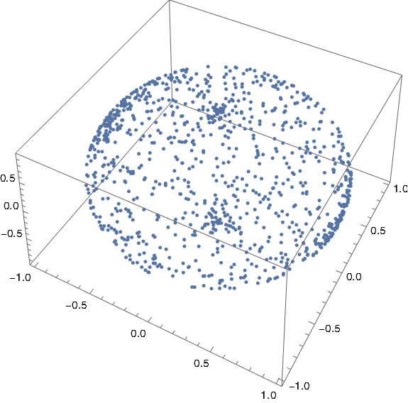
Now we’re can plot our iterates. I chose 10 + 1.9i as a starting point based on today’s date, October 19, but you could pick any non-zero starting point. And that’s kinda the point: any place you start will have the same chaotic dynamics [1].

Here’s our plotting code.

    ListPointPlot3D[
        Map[projection, NestList[latte, 10 + 1.9 I, 1000]], 
        AspectRatio -> 1]

And here’s the plot:

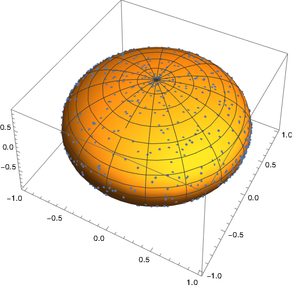
We could plot a sphere with

    SphericalPlot3D[1, {t, 0, Pi}, {ph, 0, 2 Pi}]

and stack the two plots to make it clear that the points are indeed on a sphere.

Related posts

[1] If you start with 0, you’ll next go to ∞ and stay there. But 0 and ∞ are parts of the Julia set too because the points in the neighborhoods of these points lead to chaos, no matter how small you take the open neighborhoods to be.

Quadruple factorials and Legendre functions

Last week I claimed that double, triple, and quadruple factorials came up in applications. The previous post showed how triple factorials come up in solutions to Airy’s equation. This post will show how quadruple factorials come up in solutions to Legendre’s equation.

Legendre’s differential equation is

(1-x^2) y'' - 2x y' + \nu(\nu+1)y = 0

The Legendre functions Pν and Qν are independent solutions to the equation for given values of ν.

When ν is of the form n + ½ for an integer n, the values of Pν and Qν at 0 involve quadruple factorials and also Gauss’s constant.

For example, if ν = 1/2, 5/2, 9/2, …, then Pν(0) is given by

(-1)^{(2\nu - 1)/4} \frac{\sqrt{2}(2\nu - 2)!!!!}{(2\nu)!!!!\pi g}

Source:  An Atlas of Functions

Triple factorials and Airy functions

Last week I wrote in a post on multifactorials in which I said that

Double factorials come up fairly often, and sometimes triple, quadruple, or higher multifactorials do too.

This post gives a couple examples of triple factorials in practice.

One example I wrote about last week. Triple factorial comes up when evaluating the gamma function at an integer plus 1/3. As shown here,

\Gamma\left(n + \frac{1}{3}\right) = \frac{(3n-2)!!!}{3^n} \Gamma\left(\frac{1}{3}\right)

Another example involves solutions to Airy’s differential equation

y'' - xy = 0

One pair of independent solutions consists of the Airy functions Ai(x) and Bi(x). Another pair consists of the functions

\begin{align*} f(x) &= 1 + \frac{1}{3!}x^3 + \frac{1\cdot 4}{6!}x^6 + \frac{1\cdot 4 \cdot 7}{9!}x^9 + \cdots \\ g(x) &= x + \frac{2}{4!}x^4 + \frac{2\cdot 5}{7!}x^7 + \frac{2\cdot 5 \cdot 8}{10!}x^{10} + \cdots \end{align*}

given in A&S 10.4.3. Because both pairs of functions solve the same linear ODE, each is a linear combination of the other.

Notice that the numerators are triple factorials, and so the series above can be rewritten as

\begin{align*} f(x) &= \sum_{n=0}^\infty \frac{(3n+1)!!!}{(3n+1)!} x^{3n}\\ g(x) &= \sum_{n=0}^\infty \frac{(3n+2)!!!}{(3n+2)!} x^{3n+1} \end{align*}

The next post gives an example of quadruple factorials in action.

Gauss’s constant

I hadn’t heard of Gauss’s constant until recently. I imagine I’d seen it before and paid no attention. But once I paid attention, I started seeing it more often. There’s a psychology term for this—reticular activation?—like when you buy a green Toyota and suddenly you see green Toyotas everywhere.

Our starting point is the arithmetic-geometric mean or AGM. It takes two numbers, takes the arithmetic (ordinary) mean and the geometric mean, then repeats the process over and over. The limit of this process is the AGM of the two numbers.

Gauss’s constant is the reciprocal of the AGM of 1 and √2.

g \equiv \frac{1}{\text{AGM}(1, \sqrt{2})} = 0.834626\ldots

Gauss’s constant can be expressed in terms of the Gamma function:

g = (2\pi)^{-3/2} \, \Gamma\left(\frac{1}{4}\right)^2

Exponential sums

Last week I wrote about the sum

\sum_{n=-\infty}^\infty e^{-\pi n^2} = \frac{\sqrt[4] \pi}{\Gamma\left(\frac 3 4\right)}

which we will see shortly is related to Gauss’s constant.

We can the definition of g in terms of Γ(1/4) and the reflection identify for the gamma function to show that the sum above can be written in terms of Gauss’s constant:

\sum_{n=-\infty}^\infty e^{-\pi n^2} = 2^{1/4} \sqrt{g}

The alternating version of the sum is also related to g:

\sum_{n=-\infty}^\infty (-1)^n e^{-\pi n^2} = g^2

Integrals

Another place where g comes up is in integrals of hyperbolic functions. For example

\begin{align*} \int_0^\infty \sqrt{\text{sech}(x)} \, dx &= \pi g \\ \int_0^\infty \sqrt{\text{csch}(x)} \, dx &= \sqrt{2} \pi g \end{align*}

Here

\begin{align*} \text{sech}(x) &= \frac{1}{\cosh(x)} = \frac{2}{e^x + e^{-x}} \\ \text{csch}(x) &= \frac{1}{\sinh(x)} = \frac{2}{e^x - e^{-x}} \\ \end{align*}

Beta probabilities

Another place Gauss’s constant comes up is in special values of beta distribution probabilities.

Define the incomplete beta function by

B(a, b, x) = \int_0^x t^{a-1} (1-t)^{b-1}\, dt

If X is a random variable with a beta(a, b) distribution, then the CDF of X is the normalized incomplete beta function, i.e.

\text{Prob}(X \leq x) = \frac{B(a, b, x)}{B(a, b, 1)}

A couple special values of B involve Gauss’s constant, namely

B\left(\frac{1}{4}, \frac{1}{4}, \frac{1}{2}\right) = \sqrt{2} \pi g

and

B\left(\frac{3}{4}, \frac{3}{4}, \frac{1}{2}\right) = \frac{1}{\sqrt{2} g}

Source:  An Atlas of Functions

Ubiquitous constant

The constant M defined by 1/M = √2 g is the so-called “ubiquitous constant,” though this seems like an unjustified name for such an arcane constant. Perhaps there is some context in which the constant is ubiquitous in the colloquial sense.

Gamma of integer plus one over integer

The gamma function satisfies

Γ(x+1) = x Γ(x)

and so in principle you could calculate the gamma function for any positive real number if you can calculate it on the interval (0, 1). For example,

\begin{align*} \Gamma(\pi) &= (\pi - 1)\Gamma(\pi -1) \\ &= (\pi - 1)(\pi - 2) \Gamma(\pi - 2) \\ &= (\pi - 1)(\pi - 2) (\pi - 3)\Gamma(\pi - 3) \end{align*}

So if you’re able to compute Γ(π-3) then you could compute Γ(π).

If n is a positive integer ε is some number between 0 and 1, is there a more direct way to express Γ(n + ε) in terms of Γ(ε)?

There is when ε is the reciprocal of an integer. For example,

\begin{align*} \Gamma\left(n + \frac{1}{2}\right) &= \frac{(2n-1)!!}{2^n} \Gamma\left(\frac{1}{2}\right) \\ \Gamma\left(n + \frac{1}{3}\right) &= \frac{(3n-2)!!!}{3^n} \Gamma\left(\frac{1}{3}\right) \\ \Gamma\left(n + \frac{1}{4}\right) &= \frac{(4n-3)!!!!}{4^n} \Gamma\left(\frac{1}{4}\right) \\ \end{align*}

The multiple exclamation marks may look strange if you haven’t seen this notation before. See the previous post for an explanation.

The general equation for integer k is

\Gamma\left(n + \frac{1}{k}\right) = \frac{\Pi_k(kn - k + 1)}{k^n} \Gamma\left(\frac{1}{k}\right)

where Πk is a notation for k-factorial I suggested in the previous post. A more common notation would be to put !(k) to the right of the argument rather than Πk on the left.

Here’s Python code demonstrating that the equation above holds for randomly selected n and k.

from operator import mul
from functools import reduce
from scipy.special import gamma
import numpy as np

def multifactorial(n, k):
    return reduce(mul, range(n, 0, -k), 1)

def f1(n, k):
    return gamma(n + 1/k)

def f2(n, k):
    return multifactorial(k*n - k + 1, k)*gamma(1/k)/k**n

np.random.seed(20211014)
for _ in range(1000):
    n = np.random.randint(1, 50)
    k = np.random.randint(1, 50)    
    a, b = f1(n,k), f2(n, k)
    assert( abs(a/b - 1) <= 1e-10 )

Multifactorial

The factorial of an integer n is the product of the positive integers up to n.

The double factorial of an even (odd) integer n is the product of the positive even (odd) integers up to n. For example,

8!! = 8 × 6 × 4 × 2

and

9!! = 9 × 7 × 5 × 3 × 1.

Double factorials come up fairly often, and sometimes triple, quadruple, or higher multifactorials do too.

In general, the k-factorial of n is the product of the positive integers up to n that are congruent to n mod k. Here’s how you might implement k-factorials in Python.

    from operator import mul
    from functools import reduce

    def multifactorial(n, k):
        return reduce(mul, [i for i in range(1, n+1) if (n-i)%k == 0], 1)

Update: As pointed out in the comments, multifactorial could be implemented more succinctly as

    def multifactorial(n, k):
        return reduce(mul, range(n, 0, -k), 1)

Factorial notation is a little awkward, and multifactorial notation is even more awkward. Someone seeing n!! for the first time might reasonably assume it means (n!)!, but it does not.

Adding exclamation points works, albeit awkwardly, for specific values of k, but not for variable numbers of k. One way I’ve seen to express k-factorials for variable k is to add a subscript (k) to the factorial:

n!_{(k)} \equiv n\underbrace{! \cdots !}_\text{$k$ times}

I’ve also seen the subscript on the exclamation point written as a superscript instead.

I’d like to suggest a different notation: Πk. by analogy with the Π function.

\Pi_k(n) = \prod_{\stackrel{1 \,\leq \,i \leq \,n}{i \,\equiv\, n \pmod{k}}} i

When k ≡ 1 the condition in (mod k) always holds, and we have factorial, i.e.

Π1(n) = Π(n) = n!.

One downside of this notation is that while the function Π is defined for all complex numbers (aside from singularities at negative integers) the function Πk is only defined for positive integer arguments. Still, in my opinion, this is less awkward than the alternatives I’ve seen.

By the way, the term “double factorial” seems backward. Maybe it should have been “half factorial” because you’re multiplying half as many numbers together, not twice as many. “Multifactorial” in general seems like an unfortunate name. Subfactorial might have been better, but unfortunately that name means something else.

I understand why someone may have come up with the idea of using two exclamation points for what we call double factorial; it would be hard to draw half an exclamation point. An advantage of the notation suggested here is that it suggests that there’s a variation on factorial somehow associated with k, but there’s no implication of multiplying or dividing by k.

Adding “mod k” as a subscript would be even more explicit than a subscript k. Someone who hadn’t seen

Πmod k (n)

before might be able to figure out what it means; I think they would at least easily remember what it means once told. And the presence of “mod” might suggest to the reader that the argument needs to be an integer.