Constellations in Mathematica

Mathematica has data on stars and constellations. Here is Mathematica code to create a list of constellations, sorted by the declination (essentially latitude on the celestial sphere) of the brightest star in the constellation.

constellations = EntityList["Constellation"]
sorted = SortBy[constellations, -#["BrightStars"][[1]]["Declination"] &]

We can print the name of each constellation with

Map[#["Name"] &, sorted]

This yields

{"Ursa Minor", "Cepheus", "Cassiopeia", "Camelopardalis", 
…, "Hydrus", "Octans", "Apus"}

We can print the name of the constellation along with its brightest star as follows.

Scan[Print[#["Name"], ", " #["BrightStars"][[1]]["Name"]] &, sorted]

This prints

Ursa Minor, Polaris
Cepheus, Alderamin
Cassiopeia, Tsih
Camelopardalis, β Camelopardalis
…
Hydrus, β Hydri
Octans, ν Octantis
Apus, α Apodis

Mathematica can draw star charts for constellations, but when I tried

Entity["Constellation", "Orion"]["ConstellationGraphic"]

it produced extraneous text on top of the graphic.

Related posts

Stellar magnitude

Imagine the following dialog.

“Logarithms are usually taken to integer bases, like 2 or 10.”

“What about e?”

“OK, that’s an example of an irrational base, but it’s the only one.”

“Decibels are logarithms to base 101/10.”

“Really?!”

“Yeah, you can read about this here.”

“That’s weird. But logarithms are always take to bases bigger than 1.”

“Au contraire. Bases can be less than one, not just in theory but in practice.”

This post expands on the dialog above, especially the last line. We will show that stellar magnitude is a logarithm to a base smaller than 1.

Decibles are defined as 10 times the log base 10. But as explained here, decibels are not just a multiple of a logarithm, they are logarithms, logarithms base 101/10.

Irrational bases

Raising a musical pitch a half-step (semitone) multiplies its frequency by 21/12, and so raising it 12 half-steps doubles it, raising it an octave. Semitones are logarithms base 21/12.

So here are two examples of irrational bases for logarithms: decibels are logs base 1.2589 and semitones are logs base 1.0595.

Stellar magnitude

Vega

Stellar magnitude is strange for a couple reasons. First of all, the scale runs backward to what you might expect, with brighter objects having smaller magnitude. Perhaps stellar magnitude should be called stellar dimness. But the magnitude scale made more sense when it was limited to visible stars. The most visible starts were of the first category, the next most in the second category, and the least visible in the sixth category.

Second, stellar magnitude is defined so that a change in brightness of 100 corresponds to change in magnitude of 5. This seems arbitrary until you realize the intention was to fit a scale from 1 to 100 to the magnitude of visible stars. The scale seems strange now that we apply it to a wider variety of objects than naked eye astronomy.

If a star X is 100 times as bright as a star Y, then the magnitude of X is −5 times the magnitude of Y. The log base 10 of the brightness of X is twice the log base 10 of the magnitude of Y, so magnitude is −5/2 times log base 10 of brightness.

So stellar magnitude is a multiple of log base 10, like decibels.

Now

loga(x) = logb(x) / logb(a)

for any bases a and b. If we let b = 10, this says that a multiple k of base 10 is the same as the log base a where log10(a) = 1/k, so

a = 101/k.

For decibels, k = 10, so a = 101/10 = 1.2589. For stellar magnitude, k = −5/2, so a = 10−2/5 = 0.3981.

That is, stellar magnitude is logarithm base 0.3981.

To be more precise, we need a reference point. The star Vega (image above) has magnitude 0, so the magnitude of a star is the logarithm base 0.003162 of the ratio of the star’s brightness to the brightness of Vega.

Related posts

Image of Vega by Stephen Rahn via Wikipedia.

Connecting the dots differently

A couple weeks ago I wrote about how H. A. Rey introduced a new way of looking at the constellations, making them look more like their names. That post used Leo as an example. This post looks at Boötes (The Herdsman) [1].

Here is the constellation using the connections indicated in the IAU star chart.

Bootes from IAU chart

Here is the constellation using the connections drawn in Rey’s book [2].

H. A. Rey's version of Bootes

Rey’s version adds two stars, highlighted in red, but mostly connects the same stars in a different way. I suppose the herdsman is standing in the IAU version; it’s hard to tell. In Rey’s version, the huntsman is clearly seated and smoking a pipe. This is easier to see if we rotate the image a bit.

Rey's herdsman, rotated

Here’s a comparison of the two interpretations side-by-side.

comparing both versions

Here is the Python code that produced the two images. It’s a little cleaner than the code in the earlier post, and it draws larger dots to represent brighter stars.

import matplotlib.pyplot as plt

# data from https://en.wikipedia.org/wiki/List_of_stars_in_Bo%C3%B6tes

α = (14 + 16/60, 19 + 11/60, 0.0)  
β = (15 +  2/60, 40 + 23/60, 3.5)  
γ = (14 + 32/60, 38 + 18/60, 3.0)  
δ = (15 + 16/60, 33 + 19/60, 3.5)  
ε = (14 + 45/60, 27 +  4/60, 2.3)  
ζ = (14 + 41/60, 13 + 44/60, 3.8)  
η = (13 + 55/60, 18 + 24/60, 4.5)  
θ = (14 + 25/60, 51 + 51/60, 4.0)  
κ = (14 + 13/60, 51 + 47/60, 4.5)  
λ = (14 + 16/60, 46 +  5/60, 4.2)
μ = (15 + 24/60, 37 + 23/60, 4.3)
υ = (13 + 49/60, 15 + 48/60, 4.0)  
τ = (13 + 47/60, 17 + 27/60, 4.5)  
ρ = (14 + 32/60, 30 + 22/60, 3.6)  
    
k = -15 # reverse and scale horizontal axis

def plot_star(s, m):
    plt.plot(k*s[0], s[1], m, markersize=14-2.2*s[2])    

def join(s0, s1, m='ko'):
    plot_star(s0, m)
    plot_star(s1, m)    
        
    plt.plot([k*s0[0], k*s1[0]], [s0[1], s1[1]], 'b-')    

def draw_iau():

    join(α, η)
    join(η, τ)
    join(α, ζ)
    join(α, ϵ)
    join(ϵ, δ)
    join(δ, β)
    join(β, γ)
    join(γ, λ)
    join(λ, θ)
    join(θ, κ)
    join(κ, λ)
    join(γ, ρ)
    join(ρ, α)

def draw_rey():

    join(α, η)
    join(η, υ)
    join(υ, τ)
    
    join(α, ζ)
    join(α, ϵ)
    join(ζ, ϵ)
    
    join(ϵ, δ)
    join(δ, β)
    join(δ, μ)
    join(μ, β)
    join(β, γ)
    join(γ, λ)
    join(λ, θ)
    join(θ, κ)
    join(κ, λ)
    join(γ, ρ)
    join(ρ, ϵ)

    plot_star(μ, 'r*')
    plot_star(υ, 'r*')        
    return

draw_iau()
plt.gca().set_aspect('equal')
plt.axis('off')
plt.savefig("bootes_iau.png")
plt.close()

draw_rey()
plt.gca().set_aspect('equal')
plt.axis('off')
plt.savefig("bootes_rey.png")
plt.close()

***

[1] The diaeresis over the second ‘o’ in Boötes means the two vowels are to be pronounced separately: bo-OH-tes. You may have seen the same pattern in Laocoön or oogenesis. The latter is written without a diaresis now, but I bet authors used to write it with a diaeresis on the second ‘o’.

[2] H. A. Rey. The Stars: A New Way to See Them, Second Edition.

Adding stars to constellations

Until yesterday, I was only aware of the traditional assignment of stars to constellations. In the comments to yesterday’s post I learned that H. A. Rey, best known for writing the Curious George books, came up with a new way of viewing the constellations in 1952, adding stars and connecting lines in order to make the constellations look more like their names. For example, to make Leo look more like a lion.

Book cover of Find The Constellations by H. A. Rey

The International Astronomical Union (IAU) makes beautiful star charts of the constellations, and uses Rey’s conventions, sorta.

This post will look at the example of Leo, from the IAU chart and from Rey’s book Find The Constellations.

(I wonder whether the ancients also added stars to what we received as the traditional versions of constellations. Maybe they didn’t consciously notice the other stars. Or maybe they did, but only saw the need to record the brightest stars, something like the way Hebrew only recorded the consonants of words.)

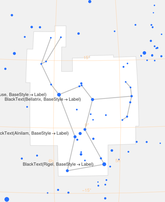
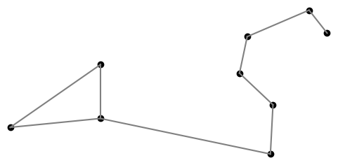
Here is the IAU star chart for Leo, cropped to just show the constellation graph. (The white region is Leo-as-region and the green lines are Leo-as-graph.)

Leo star chart IAU

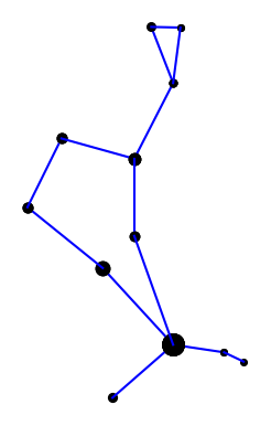
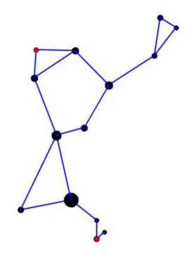
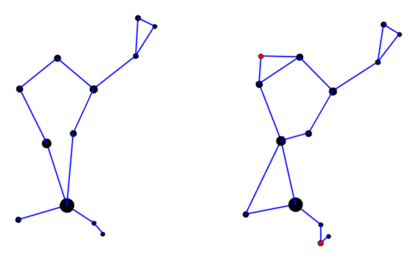
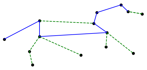
Rey’s version of Leo is a little different. Here is my attempt to reproduce Rey’s version from page 9 of Find the Constellations.

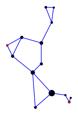
And for comparison, here’s my reproduction of the IAU version.

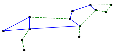
The solid blue lines are traditional. The dashed green lines were added by Rey and the IAU respectively.

Here is the Python code that produced the two images. Star names and coordinates are explained in the previous post.

# data from https://en.wikipedia.org/wiki/List_of_stars_in_Leo
import matplotlib.pyplot as plt

# star coordinates
δ = (11 + 14/60, 20 + 41/60)  
β = (11 + 49/60, 14 + 34/60)  
θ = (11 + 14/60, 15 + 26/60)  
α = (10 +  8/60, 11 + 58/60)  
η = (10 +  7/60, 16 + 46/60)  
γ = (10 + 20/60, 19 + 51/60)  
ζ = (10 + 17/60, 23 + 25/60)  
μ = ( 9 + 53/60, 26 +  0/60)  
ε = ( 9 + 46/60, 23 + 46/60)  
κ = ( 9 + 25/60, 26 + 11/60)  
λ = ( 9 + 32/60, 22 + 58/60)  
ι = (11 + 24/60, 10 + 32/60)  
σ = (11 + 21/60,  6 +  2/60)
ο = ( 9 + 41/60,  9 + 54/60)
ρ = (10 + 33/60,  9 + 18/60)

k = -20 # reverse and scale horizontal axis

def plot_stars(ss):
    for s in ss:
        plt.plot(k*s[0], s[1], 'ko')
    
def join(s0, s1, style, color):
    plt.plot([k*s0[0], k*s1[0]], [s0[1], s1[1]], style, color=color)    

def draw_iau():
    plot_stars([δ,β,θ,α,η,γ,ζ,μ,ε,κ,λ,ι,σ])        

    # traditional
    join(δ, β, '-', 'b')
    join(β, θ, '-', 'b')
    join(θ, η, '-', 'b')
    join(η, γ, '-', 'b')
    join(γ, ζ, '-', 'b')
    join(ζ, μ, '-', 'b')
    join(μ, ε, '-', 'b')
    join(δ, θ, '-', 'b')
    
    # added
    join(θ, ι, '--', 'g')
    join(ι, σ, '--', 'g')
    join(δ, γ, '--', 'g')
    join(ε, η, '--', 'g')
    join(μ, κ, '--', 'g')
    join(κ, λ, '--', 'g')
    join(λ, ε, '--', 'g')
    join(η, α, '--', 'g')

def draw_rey():
    plot_stars([δ,β,θ,α,η,γ,ζ,μ,ε,λ,ι,σ, ρ,ο])        

    # traditional
    join(δ, β, '-', 'b')
    # join(β, θ, '-', 'b')
    join(θ, η, '-', 'b')
    join(η, γ, '-', 'b')
    join(γ, ζ, '-', 'b')
    join(ζ, μ, '-', 'b')
    join(μ, ε, '-', 'b')
    join(δ, θ, '-', 'b')
    
    # added
    join(θ, ι, '--', 'g')
    join(ι, σ, '--', 'g')
    join(δ, γ, '--', 'g')
    join(λ, ε, '--', 'g')
    join(η, α, '--', 'g')
    join(λ, ε, '--', 'g')
    join(θ, ρ, '--', 'g')
    join(η, ο, '--', 'g')

Plotting constellations

Suppose you wanted to write a program to plot constellations. This leads down some interesting rabbit trails.

When you look up data on stars in constellations you run into two meanings of constellation. For example, Leo is a region of the night sky containing an untold number of stars. It is also a pattern of nine particular stars connected by imaginary lines. It’s easier to find data on the former, say sorted by brightness.

Are the nine brightest stars in Leo-the-region the nine stars of Leo-the-stick-figure? Not exactly, but close.

Wikipedia has an article that list stars in each constellation region, and star charts that have constellations as stick figures. If the stars on the chart are labeled, you can cross reference them with Wikipedia.

On a particular star chart I have, the stars in Leo are labeled with their Bayer designation. Roughly speaking the Bayer designation labels the stars within a constellation with Greek letters in descending order of brightness, but there are inconsistencies. The nomenclature goes back to Johann Bayer (1572–1625) and has its flaws.

The stars in Leo, in line-drawing order, are

  1. δ Leo
  2. Denebola (β Leo)
  3. θ Leo
  4. Regulus (α Leo)
  5. η Leo
  6. γ Leo
  7. ζ Leo
  8. μ Leo
  9. ε Leo

You can look up the coordinates of these stars here. Line-drawing order does not correspond to brightness order, so without a labeled star chart you’d have some research to do. My chart labels all the stars in Leo (the stick figure), but not, for example, in Virgo.

γ Leo is actually two stars, and Wikipedia ranks the brightness of the stars a little differently than Bayer did, which is understandable since brightness could not be objectively measured in his day. Wikipedia also inserts a few stars in between the stars listed above.

Here’s a plot of Leo using the data referenced above.

Dutton’s Navigation and Piloting

This morning Eric Berger posted a clip from The Hunt for Red October as a meme, and that made me think about the movie.

I watched Red October this evening, for the first time since around the time it came out in 1990, and was surprised by a detail in one of the scenes. I recognized one of the books: Dutton’s Navigation and Piloting.

Screen shot with Dutton's Navigation and Piloting

I have a copy of that book, the 14th edition. The spine looks exactly the same. The first printing was in 1985, and I have have the second printing from 1989. So it is probably the same edition and maybe even the same printing as in the movie. I bought the book last year because it was recommended for something I was working on. Apparently it’s quite a classic since someone thought that adding a copy in the background would help make a realistic set for a submarine.

My copy has a gold sticker inside, indicating that the book came from Fred L. Woods Nautical Supplies, though I bought my copy used from Alibris.

Here’s a clip from the movie featuring Dutton’s.

Dutton’s has a long history. From the preface:

Since the first edition of Navigation and Nautical Astronomy (as it was then titled) was written by Commander Benjamin Dutton, U. S. Navy, and published in 1926, this book has been updated and revised. The title was changed after his death to more accurately reflect its focus …

The 14th edition contains a mixture of classical and electronic navigation, navigating by stars and by satellites. It does not mention GPS; that is included in the latest edition, the 15th edition published in 2003.

Related posts

What exactly is a day?

How many days are in a year? 365.

How many times does the earth rotate on its axis in a year? 366.

If you think a day is the time it takes for earth to rotate once around its axis, you’re approximately right, but off by about four minutes.

What we typically mean by “day” is the time it takes for earth to return to the same position relative to the sun, i.e. the time from one noon to the next. But because the earth is orbiting the sun as well as rotating on its axis, it has to complete a little more than one rotation around its axis to bringsi the sun back to the same position.

Since there are approximately 360 days in a year, the earth has to rotate about 361 degrees to bring the sun back into the same position. This extra rotation takes 1/360th of a day, or about 4 minutes. (We’ll be more precise below.)

Here’s another way to see that the number of rotations has to be more than the number days in a year. To make the numbers simple, assume there are 360 days in a year. Suppose you’re looking up at the noon sun one day. Next suppose it is exactly 180 days later and the earth had rotated 180 times. Because the earth is on the opposite side of the sun, you would be on the opposite side of the sun too. For it to be noon again 180 days later, the earth would have to have made 180.5 rotations, making 361 rotations in a 360-day year.

Sidereal days

Imagine an observer looking straight down at the Earth’s north pole from several light years away. Imagine also an arrow from the center of the Earth to a fixed point on the equator. The time it takes for the observer to see that arrow return to same angle is a sidereal day. The time it takes for that arrow to go from pointing at the sun to pointing at the sun again is a solar day, which is about four minutes longer [1].

If you assume a year has 365.25 (solar) days, but also assume Earth is in a circular orbit around the sun, you’ll calculate a sidereal day to be about 3 minutes and 57 seconds shorter than a solar day. Taking the elliptical shape of Earth’s orbit into account takes about a second off that amount.

More astronomy posts

[1] Technically this is an apparent solar day, a solar day from the perspective of an observer. The length of an apparent solar day varies through the year, but we won’t go into that here.

Planets evenly spaced on log scale

The previous post was about Kepler’s observation that the planets were spaced out around the sun the same way that nested regular solids would be. Kepler only knew of six planets, which was very convenient because there are only five regular solids. In fact, Kepler thought there could only be six planets because there are only five regular solids.

The distances to each of the planets is roughly a geometric series. Ratios of consecutive distances are between 1.3 and 3.4. That means the distances should be fairly evenly spaced on a logarithmic scale. The plot below shows that this is the case.

Distance to planets in our solar system on log scale

The plot goes beyond the six planets known in Kepler’s day and adds four more: Uranus, Neptune, Pluto, and Eris. Here I’m counting the two largest Kuiper belt objects as planets. Distances are measured in astronomical units, i.e. Earth = 1.

Update: The fit is even better if we include Ceres, the largest object in the asteroid belt. It’s now called a dwarf planet, but it was considered a planet for the first fifty years after it was discovered.

Distances in our solar system including planets and dwarf planets

Extrasolar planets

Is this just true of our solar system, or is it true of other planetary systems as well? At the time of writing, we know of one planetary system outside our own that has 8 planets. Three other systems have around 7 planets; I say “around” because it depends on whether you include unconfirmed planets. The spacing between planets in these other systems is also fairly even on a logarithmic scale. Data on planet distances is taken from each system’s Wikipedia page. Distances are semimajor axes, not average distances.

This post just shows plots. See this follow up post for regression results.

Kepler-90

Kepler-90 is the only planetary system outside our own with eight confirmed planets that we know of.

Distances to planets in Kepler-90 system

HD 10180

HD 10180 has seven confirmed planets and two unconfirmed planets. The unconfirmed planets are included below, the 3rd and 6th objects.

Distances to planets in HD 10180 system

HR 8832

The next largest system is HR 8832 with five confirmed planets and two unconfirmed, numbers 5 and 6 below. It would work out well for this post if the 6th object were found to be a little closer to its star.

Distances to planets in HR 8832 system

TRAPPIST-1

TRAPPIST-1 is interesting because the planets are very close to their star, ranging from 0.01 to 0.06 AU. Also, this system follows an even logarithmic spacing more than the others.

Distances to planets in TRAPPIST-1 system

Systems with six planets

There are currently four known systems with four planets: Kepler-11, Kepler-20, HD 40307, and HD 34445. They also appear to have planets evenly spaced on a log scale.

Distances between planets in known systems with six planets

Like TRAPPIST-1, Kepler-20 has planets closer in and more evenly spaced (on a log scale).

More astronomy posts

Planets and Platonic solids

Johann Kepler discovered in 1596 that the ratios of the orbits of the six planets known in his day were the same as the ratios between nested Platonic solids. Kepler was understandably quite impressed with this discovery and called it the Mysterium Cosmographicum.

Kepler's Mysterium Cosmographicum

I heard of this in a course in the history of astronomy long ago, and have had in the back of my mind that one day I’d look into this in detail. How exactly do you fit these regular solids together? How well do the planetary ratios match the regular solid ratios?

Imagine the orbit of each planet being the equator of a spherical shell centered at the sun. The five regular solids fit snugly into the spaces between the shells. Between Mercury and Venus you can insert an octahedron. Its inradius is the distance of Mercury to the sun, and its circumradius is the distance of Venus to the sun. You can fit the other regular solids in similarly, the icosahedron between Venus and Earth, the dodecahedron between Earth and Mars, the tetrahedron between Mars and Jupiter, and the hexahedron (cube) between Jupiter and Saturn.

Here’s the data on the inradius and circumradius of each regular solid taken from Mathworld.

    |--------------+--------------+----------|
    | solid        | circumradius | inradius |
    |--------------+--------------+----------|
    | octahedron   |      0.70722 |  0.40825 |
    | icosahedron  |      0.95106 |  0.75576 |
    | dodecahedron |      1.40126 |  1.11352 |
    | tetrahedron  |      0.61237 |  0.20412 |
    | hexahedron   |      0.86603 |  0.50000 |
    |--------------+--------------+----------|

Here’s the data on average orbit radii measured in astronomical units taken from WolframAlpha.

    |---------+----------|
    | Planet  | Distance |
    |---------+----------|
    | Mercury |  0.39528 |
    | Venus   |  0.72335 |
    | Earth   |  1.00000 |
    | Mars    |  1.53031 |
    | Jupiter |  5.20946 |
    | Saturn  |  9.55105 |
    |---------+----------|

So how well does Kepler’s pattern hold? In the table below, “Planet ratio” is the radius ratios of Venus to Mercury, Earth to Venus, etc. “Solid ratio” is the circumradius to inradius ratio of the regular solids in the order given above.

    |--------------+-------------|
    | Planet ratio | Solid ratio |
    |--------------+-------------|
    |      1.82997 |     1.73205 |
    |      1.38246 |     1.25841 |
    |      1.53031 |     1.25841 |
    |      3.40419 |     3.00000 |
    |      1.83340 |     1.73205 |
    |--------------+-------------|

Not a bad fit, but not great either. I’ve heard that the fit was better given the data available to Kepler at the time; if Kepler had had more accurate data, he might not have come up with his Mysterium Cosmographicum.

By the way, notice some repetition in the solid ratios. The implied equalities are exact. The icosahedron and dodecahedron have the same ratio of circumradius to inradius because they are dual polyhedra. The same is true for the cube and the octahedron. Also, the ratio of 3 for the tetrahedron is exact.

Update: What if Kepler had known about more planets? The next planet ratios in our table above would be 2.01, 1.57, and 1.35. None of these is close to any of the solid ratios.

More polyhedra posts

Mathematical modeling in Milton

In Book VIII of Paradise Lost, the angel Raphael tells Adam what difficulties men will have with astronomy:

Hereafter, when they come to model heaven
And calculate the stars: how they will wield the
The mighty frame, how build, unbuild, contrive
To save appearances, how gird the sphere
With centric and eccentric scribbled o’er,
Cycle and epicycle, orb in orb.


Related post Quaternions in Paradise Lost