Total curvature of a knot

Posted on 1 October 2019 by John

Tie a knot in a rope and join the ends together. At each point in the rope, compute the curvature, i.e. how much the rope bends, and integrate this over the length of the rope. The Fary-Milnor theorem says the result must be greater than 4π. This post will illustrate this theorem by computing numerically integrating the curvature of a knot.

If p and q are relatively prime integers, then the following equations parameterize a knot.

x(t) = cos(pt) (cos(qt) + 2)
y(t) = sin(pt) (cos(qt) + 2)
z(t) = -sin(qt)

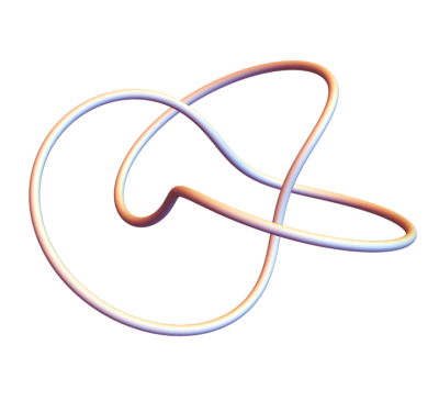
This is in fact a torus knot because the curve stays on the surface of a torus (doughnut) [1]. We can get a trefoil knot, for example, by setting p = 2 and q = 3.

Trefoil knot

We’ll use Mathematica to compute the total curvature of this knot and other examples. First the parameterization:

    x[t_, p_, q_] := Cos[p t] (Cos[q t] + 2)
    y[t_, p_, q_] := Sin[p t] (Cos[q t] + 2) 
    z[t_, p_, q_] := -Sin[q t]

We can plot torus knots as follows.

    k[t_, p_, q_] := { 
        x[t, p, q], 
        y[t, p, q], 
        z[t, p, q]
    }
    Graphics3D[Tube[Table[k[i, p, q], {i, 0, 2 Pi, 0.01}], 
        0.08], Boxed -> False]

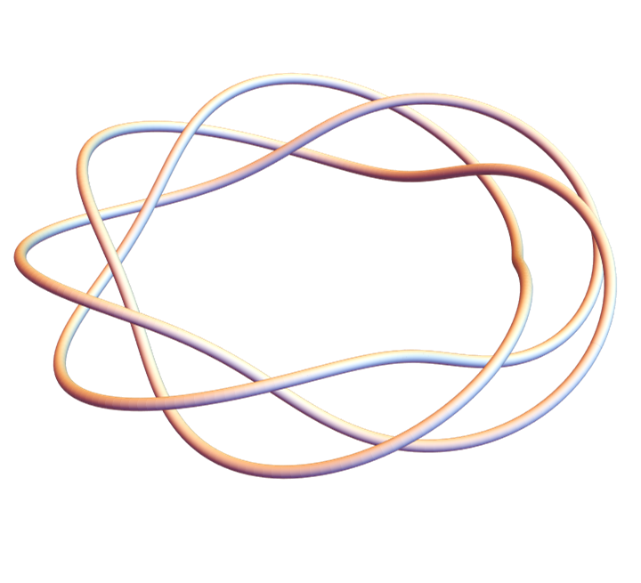
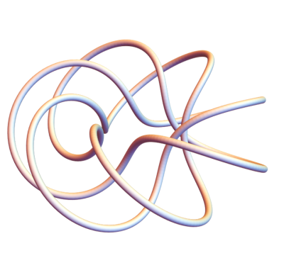
Here’s a more complicated knot with p = 3 and q = 7.

(3, 7) knot

Before we can integrate the curvature with respect to arc length, we need an expression for an element of arc length as a function of the parameter t.

    ds[t_, p_, q_] :=  Sqrt[ 
        D[x[t, p, q], t]^2 + 
        D[y[t, p, q], t]^2 + 
        D[z[t, p, q], t]^2
    ]

Now we can compute the total curvature.

    total[p_, q_] := NIntegrate[
        ArcCurvature[k[t, p, q], t] ds[t, p, q], 
        {t, 0, 2 Pi}
    ]

We can use this to find that the total curvature of the (2,3) torus knot, the trefoil, is 17.8224, whereas 4π is 12.5664. So the Fary-Milnor theorem holds.

Let’s do one more example, this time a (1,4) knot.

unknot

You can see that this is not actually knot. This doesn’t contradict what we said above because 1 divides 4. When p or q equal 1, we get an unknot.

When we compute its total curvature we get 24.2737, more than 4π. The Fary-Milnor theorem doesn’t say that total curvature in excess of 4π is a sufficient condition for a loop to be knotted; it says it’s necessary. Total curvature less than 4π proves that something isn’t a knot, but curvature greater than 4π doesn’t prove anything.

More on curvature and knots

[1] If you change out the 2s in the parameterization with a larger number, it’s easier to see from the graphs that the curves are on a torus. For example, if we plot the (3,7) knot again, replacing 2’s in the definition of x(t) and y(t) with 5’s, we can kinda see a torus inside the knot.

(3, 7) knot torus

Unit speed curve parameterization

Posted on 15 July 2018 by John

A friend asked me a question the other day that came out of a graphics application. He needed to trace out an ellipse in such a way that the length of curve traced out each second was constant. For a circle, the problem is simple: (cos(t), sin(t)) will trace out a circle covering a constant amount of arc length per unit time. The analogous parameterization for an ellipse, (a cos(t), b sin(t)) will move faster near the longer semi-axis and slower near the shorter one.

There’s a general solution to the problem for any curve. Given a parameterization p(t), where p is vector-valued, the length covered from time 0 to time t is

$s(t) = \int_0^t || p'(\tau) || \,d\tau$

If you change the time parameterization by inverting this function, solving for t as a function of s, then the total length of curve traversed by p(t(s)) up to time s is s. This is called either the unit speed parameterization or parameterization by arc length.

The hard part is inverting s(t). If you had to find a unit speed parameterization in a calculus class, the problem would be carefully designed so the function s(t) is easy to invert. Real applications don’t usually work out so easily.

Digression on elliptic integrals and elliptic functions

My response to my friend’s question was that there probably is a closed-form unit speed parameterization, but it would probably involve elliptic functions. He didn’t need much resolution, and decided to do something ad hoc.

Starting with the parameterization p(t) = (a cos(t), b sin(t)), the arc length s(t) is given by a special function known as an “incomplete elliptic integral of the second kind.” I remembered that the Jacobi elliptic functions were related to the inverses of elliptic integrals, so my hunch was that you could make a unit speed parameterization using Jacobi elliptic functions. Maybe you can, but it’s not as easy as I thought because the Jacobi functions are related to the inverses of elliptic integrals of the first kind.

Elliptic integrals are so named because they were first identified by computing arc length for a (portion of) an ellipse. Elliptic functions were discovered by inverting elliptic integrals, but not the same class of elliptic integrals that give the arc length of an ellipse. (There may well be a transformation that makes these more directly related, but I’m not aware of it.)

Incidentally, elliptic curves are related to elliptic functions, but they are not ellipses! There is a connection from ellipses to elliptic curves, but it’s historical and indirect.

What if we had a more general curve than an ellipse, say something parameterized by cubic splines? Cubic splines are piecewise cubic polynomials, patched together in such a way that the first and second derivatives are continuous across the patches. We can find length of a spline by finding the length of each polynomial patch.

If p(t) is the parameterization of a curve in 2 or 3 dimensions (or really any number of dimensions) and each component of p is a cubic polynomial, then each component of the derivative of p is a quadratic polynomial, and so the sum of the squares of the components is a fourth degree polynomial. So finding the arc length involves integrating the square root of a fourth degree polynomial. This makes it an elliptic integral!

Unfortunately, knowing that the arc length of a cubic spline corresponds to an elliptic integral is not so useful because it could be any type of elliptic integral, depending on its parameters. You’d have to do some work first to put it into a form where you could call on elliptic integrals to finish your problem.

Numerically computing arc length and unit speed parameterization

The elliptic integral path is something of a dead end. It could still be useful if you needed high accuracy, or if you had some restriction on the class of curves you’re interested in. But in general, you’d need to use numerical integration to find the arc length.

You could also find unit-speed parameterizations numerically, using root-finding to invert s(t) at particular points. Since s is an increasing function of t, you could use a bisection method, which is not the most efficient approach but very robust.

It takes a fair amount of computation to carry root finding where each function evaluation requires computing a numerical integral. But this would work, and depending on your context it could be efficient enough.

If you needed more efficiency, say for a real-time embedded system, you could take a different approach. Your spline is probably an approximation to something else, and so your solution only needs to be as accurate as the spline approximation. This gives you the wiggle room to do something more efficient. You might change your parameterization slightly to make the arc length calculations easier, or come up with a way to approximately invert the arc length function, something that takes advantage of your particular problem and error tolerance.

Curvature and automatic differentiation

Posted on 30 March 2018 by John

Curvature is tedious to calculate by hand because it involves calculating first and second order derivatives. Of course other applications require derivatives too, but curvature is the example we’ll look at in this post.

Computing derivatives

It would be nice to write programs that only explicitly implement the original function and let software take care of finding the derivatives.

Numerical differentiation

Finite difference approximations for derivatives are nothing new. For example, Euler (1707–1783) used finite differences to numerically solve differential equations. But numerical differentiation can be inaccurate or unstable, especially for higher order derivatives.

Symbolic differentiation

Symbolic differentiation is another approach, having the computer manipulate expressions much as a person would do by hand. It works well for many problems, though it scales poorly for large problems. It also requires functions to be presented in traditional mathematical form, not in the form of source code.

Automatic differentiation

Automatic differentiation is a third way. Like numerical differentiation, it works with floating point numbers, not symbolic expressions. But unlike numerical differentiation, the result does not have approximation error.

As someone put it, automatic differentiation applies the chain rule to floating point numbers rather than to symbolic expressions.

Python implementation

I’ll use the Python library autograd to compute curvature and illustrate automatic differentiation. autograd is not the most powerful automatic differentiation library for Python, but it is the simplest I’ve seen.

We will compute the curvature of a logistic curve.

$y = \frac{1}{1 + e^{-x}}$

The curvature of the graph of a function is given by

$\kappa(x) = \frac{|y''|}{(1 + y'^2)^{3/2}}$

Here’s Python code using autograd to compute the curvature.

    import autograd.numpy as np
    from autograd import grad

    def f(x):
        return 1/(1 + np.exp(-x))

    f1 = grad(f)  # 1st derivative of f
    f2 = grad(f1) # 2nd derivative of f

    def curvature(x):
        return abs(f2(x))*(1 + f1(x)**2)**-1.5

Curvature plots

The graph is relatively flat in the middle and at the far ends. In between, the graph bends creating two regions of higher curvature.

    import matplotlib.pyplot as plt

    x = np.linspace(-5, 5, 300)
    plt.plot(x, f(x))
    plt.xlabel("$x$")
    plt.ylabel("$y$")
    plt.title("Logistic curve")
    plt.savefig("logistic_curve.svg")

Now let’s look at the curvature.

    y = [curvature(t) for t in x]
    plt.plot(x, y)
    plt.xlabel("$x$")
    plt.ylabel(r"$\kappa(x)$")
    plt.title("Curvature")
    plt.savefig("plot_logistic_curvature.svg")

curvature for logistic curve

As we should expect, the curvature is small at the ends and in the middle, with local maxima in between.

We can also look at the signed curvature, the same expression as curvature but without the absolute value.

$k(x) = \frac{y''}{(1 + y'^2)^{3/2}}$

We plot this with the following code.

    def signed_curvature(x):
        return f2(x)*(1 + f1(x)**2)**-1.5

    y = [signed_curvature(t) for t in x]
    plt.plot(x, y)
    plt.xlabel("$x$")
    plt.ylabel(r"$k(x)$")
    plt.title("Signed curvature")
    plt.savefig("graph_signed_curvature.svg")

The result looks more like a sine wave.

The positive values mean the curve is bending counterclockwise, and the negative values mean the curve is bending clockwise.

Related post: Squircles and curvature

Apple design, squircles, and curvature

Posted on 13 February 2018 by John

A “squircle” is a sort of compromise between a square and circle, but one that differs from a square with rounded corners. It’s a shape you’ll see, for example, in some of Apple’s designs.

squircle

A straight line has zero curvature, and a circle with radius r has curvature 1/r. So in a rounded square the curvature jumps from 0 to 1/r where the flat side meets the circular corner. But in the figure above there’s no abrupt change in curvature but instead a smooth transition. More on that in just a bit.

To get a smoother transition from the corners to the flat sides, designers use what mathematicians would call L^p balls, curves satisfying

|x|^p + |y|^p = 1

in rectangular coordinates or

$r = \frac{1}{\left(|\cos \theta|^p + |\sin \theta|^p \right)^{1/p}}$

in polar coordinates.

When p = 2 we get a circle. When p = 2.5, we get square version of the superellipse. As p increases the corners get sharper, pushing out toward the corner of a square. Some sources define the squircle to be the case p = 4 but others say p = 5. The image at the top of the post uses p = 4. [*]

To show how the curvature changes, let’s plot the curvature on top of the squircle. The inner curve is the squircle itself, and radial distance to the outer curve is proportional to the curvature.

Here’s the plot for p = 4.

curvature p = 4

And here’s the plot for p = 5.

curvature p = 5

If we were to make the same plot for a rounded square, the curvature would be zero over the flat sides and jump to some constant value over the circular caps. We can see above that the curvature is largest over the corners but continuously approaches zero toward the middle of the sides.

Easter eggs and yellow pigs

Posted on 25 January 2018 by John

An Easter egg is a hidden feature, a kind of joke. The term was first used in video games but the idea is broader and older than that. For example, Alfred Hitchcock made a brief appearance in all his movies. And I recently heard that there’s a pineapple or reference to a pineapple in every episode of the television show Psych.

Michael Spivak put references to “yellow pig” in some of his books. I’ve heard that he put allusions to yellow pigs in all his books, but I don’t have all his books, and I haven’t been able to find yellow pigs in two of his books that I do own.

Spivak’s calculus text is dedicated to the memory of Y. P.

Dedicated to the Memory of Y. P.

If you look up yellow pig in the index of the book, it will take you to a page that makes a passing reference to “whole hog.”

Spivak’s publishing company, Publish or Perish Press, originally used a pig as part of its logo.

Publish or Perish old logo

The website now has no logo. His most recent book, Physics for Mathematicians: Mechanics I, uses a different logo.

The cover of Spivak’s Differential Geometry, Volume 1, second edition, has two yellow drawings of a pig.

Cover of Spivak's Differential Geometry, Volume 1, second edition

If you look up yellow pig in the index, it takes you to a page that doesn’t mention pigs, but does include a drawing that looks something like a ham.

Ham-like illustration from Spivak's Differential Geometry, volume 1

I do not see a reference to yellow pig in Spivak’s first book, Calculus on Manifolds. It was published by Benjamin Cummings. Maybe they would not allow Easter eggs, or maybe the idea of including Easter eggs didn’t occur to Spivak until he had his own publishing company. I also do not see a reference to yellow pigs in his recent Physics for Mathematicians book.

One of my favorite proofs: Lagrange multipliers

Posted on 27 September 2016 by John

One of my lightbulb moments in college was when my professor, Jim Vick, explained the Lagrange multiplier theorem. The way I’d seen it stated in a calculus text gave me no feel for why it should be true, but his explanation made sense immediately.

Suppose f(x) is a function of several variables, i.e. x is a vector, and g(x) = c is a constraint. Then the Lagrange multiplier theorem says that at the maximum of f subject to the constraint g we have ∇f = λ ∇g.

Where does this mysterious λ come from? And why should the gradient of your objective function be related to the gradient of a constraint? These seem like two different things that shouldn’t even be comparable.

Here’s the geometric explanation. The set of points satisfying g(x) = c is a surface. And for any k, the set of points satisfying f(x) = k is also surface. Imagine k very large, larger than the maximum of f on the surface defined by g(x) = c. You could think of the surface g(x) = c being a balloon inside the larger balloon f(x) = k.

Now gradually decrease k, like letting the air out of the outer balloon, until the surfaces g(x) = c and f(x) = k first touch. At that point, the two surfaces will be tangent, and so their normal vectors, given by their gradients, point in the same direction. That is, ∇f and ∇g are parallel, and so ∇f is some multiple of ∇g. Call that multiple λ.

I don’t know how well that explanation works when written down. But when I heard Jim Vick explain it, moving his hands in the air, it was an eye-opener.

This is not a rigorous proof, and it does not give the most general result possible, but it explains what’s going on. It’s something to keep in mind when reading proofs that are more rigorous or more general. As I comment on here,

Proofs serve two main purposes: to establish that a proposition is true, and to show why it is true.

The literally hand-wavy proof scores low on the former criterion and high on the latter.

***

Jim Vick was a great teacher. Some of us affectionately called him The Grinning Demon because he was always smiling, even while he gave devilishly hard homework. He was Dean of Natural Sciences when I took a couple classes from him. He later became Vice President for Student Affairs and kept teaching periodically. He has since retired but still teaches.

After taking his topology course, several of us asked him to teach a differential geometry course. He hesitated because it’s a challenge to put together an undergraduate differential geometry course. The usual development of differential geometry uses so much machinery that it’s typically a graduate-level course.

Vick found a book that starts by looking only at manifolds given by level sets of smooth functions, like the surfaces discussed above. Because these surfaces sit inside a Euclidean space, you can quickly get to some interesting geometric results using elementary methods. We eventually got to the more advanced methods, but by then we had experience in a more tangible setting. As Michael Atiyah said, abstraction should follow experience, not precede it.

Covariant and contravariant

Posted on 28 February 2013 by John

The terms covariant and contravariant come up in many contexts. An earlier post discussed how the terms are used in programming and category theory. The meaning in programming is an instance of the general use in category theory.

Vector fields can be covariant or contravariant too. This is also an instance of the categorical usage, except the terminology is backward.

Michael Spivak explains:

Nowadays such situations are always distinguished by calling the things which go in the same direction “covariant” and the things which go in the opposite direction “contravariant.” Classical terminology used these same words, and it just happens to have reversed this: a vector field is called a contravariant vector field, while a section of T*M is called a covariant vector field. And no one had the gall or authority to reverse terminology sanctified by years of usage. So it’s very easy to remember which kind of vector field is covariant, and which is contravariant — it’s just the opposite of what it logically ought to be.

Emphasis added.

In defense of classical nomenclature, it was established decades before category theory. And as Spivak explains immediately following the quotation above, the original terminology made sense in its original context.

From Spivak’s Differential Geometry, volume 1. I own the 2nd edition and quoted from it. But it’s out of print so I linked to the 3rd edition. I doubt the quote changed between editions, but I don’t know.

Related: Applied category theory

Differential geometry