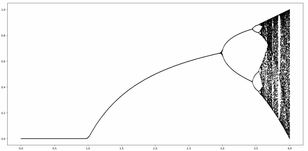
The last four post have looked at the bifurcation diagram for the logistic map.

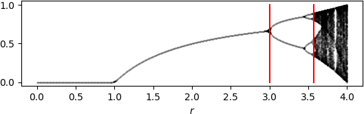
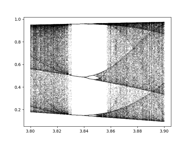
There was one post on the leftmost region, where there is no branching. Then two posts on the region in the middle where there is period doubling. Then a post about the chaotic region in the end.

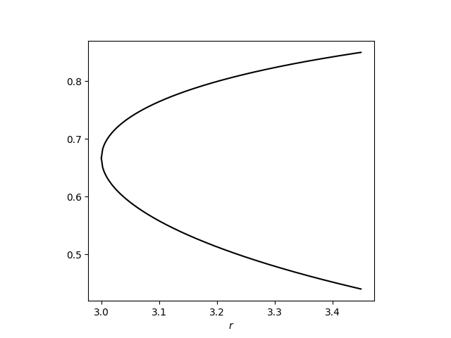
This post returns the middle region. Here’s an image zooming in on the first three forks.

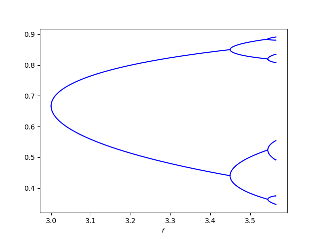
The nth region in the period doubling region has period 2ⁿ.

I believe, based on empirical results, that in each branching region, the branches are visited in the same order. For example, in the region containing r = 3.5 there are four branches. If we number these from bottom to top, starting with for the lowest branch, I believe a point on branch 0 will go to a point on branch 2, then branch 1, then branch 3. In summary, the cycle order is [0, 2, 1, 3].

Here are the cycle orders for the next three regions.

[0, 4, 6, 2, 1, 5, 3, 7]

[0, 8, 12, 4, 6, 14, 10, 2, 1, 9, 13, 5, 3, 11, 7, 15]

[0, 16, 24, 8, 12, 28, 20, 4, 6, 22, 30, 14, 10, 26, 18, 2, 1, 17, 25, 9, 13, 29, 21, 5, 3, 19, 27, 11, 7, 23, 15, 31]

[0, 32, 48, 16, 24, 56, 40, 8, 12, 44, 60, 28, 20, 52, 36, 4, 6, 38, 54, 22, 30, 62, 46, 14, 10, 42, 58, 26, 18, 50, 34, 2, 1, 33, 49, 17, 25, 57, 41, 9, 13, 45, 61, 29, 21, 53, 37, 5, 3, 35, 51, 19, 27, 59, 43, 11, 7, 39, 55, 23, 15, 47, 31, 63]

Two questions:

1. Is the cycle order constant within a region of a constant period?
2. If so, what can be said about the order in general?

I did a little searching into these questions, and one source said there are no known results along these lines. That may or may not be true, but it suggests these are not common questions.

The last couple posts have been looking at the logistic bifurcation diagram a little at a time.

The first post in the series looked at the details of that part of the diagram that looks like the graph of a function, where there parameter r in the logistic map

f(x) = r x(1 − x)

varies from o to 3.

The first branch point occurs at r = 3. When r is exactly equal to 3, almost all starting points converge to the same point, though they converge very slowly. When r is slightly larger than 3 the (stable) iterates no longer converge to a point but instead oscillate between two points.

The second post in this series looked at the first fork, corresponding to values of r from 3 to 1 + √6. For r larger than 1 + √6 the previous stable cycle points become unstable and split into two new cycles each. These new cycles will split (“bifurcate”) into two new cycles, and so on and so on until there are infinitely many cycles and chaos breaks out around r = 3.56995.

This post will look at the horizontal spacing between branch points.

The first branch point occurs when r equals b₁ = 3.

The two branches branch again when r crosses b₂ = 1 + √6.

The next branch point is b₃ = 3.5440903…. Why is there a simple expression for b₁ and b₂ but not for b₃? Everything gets more complicated as r increases. The number b₃ is algebraic, the root of a 12th degree polynomial [1].

t¹² − 12t¹¹ + 48t¹⁰ − 40t⁹ − 193t⁸ + 392t⁷ + 44t⁶ + 8t⁵ − 977t⁴ − 604t³ + 2108t² + 4913 = 0

The number b₄ has algebraic also been shown to be algebraic: someone found a 120-degree polynomial with integer coefficients such that −b₄(b₄ − 2) is a root [1]. The coefficients in the polynomial vary over 72 orders of magnitude. Perhaps its possible to find polynomials with other branch points as roots, but this doesn’t seem promising or practical.

The spacing between branch points decreases rapidly, becoming infinitely small before chaos breaks out. The ratio of spacings between consecutive branch points converges to a constant, known as Feigenbaum’s constant

δ = 4.66920…

This constant is known to surprising precision. Directly computing the constant to high precision by numerically finding branch points would be impractical, but Feigenbaum came up with an indirect way of computing his constant via a functional equation. The constant δ has been computed at least 1018 digits.

Feigenbaum’s constant does not just apply to the iterations of the logistic map. It’s a “universal” constant in that it applies to a class of dynamical systems.

Previous posts in this series

• The simple part of the logistic map isn’t that simple
• The first fork

[1] Jonathan Borwein and David Bailey. Mathematics by Experiment: Plausible Reasoning in the 21st Century. 2004.

The previous post looked at iterations of the logistic map

f(x) = r x(1 − x)

for 0 ≤ r ≤ 3. This post will look at the range 3 ≤ r ≤ 1 + √6. If you’re not familiar with the logistic map I’d suggest reading the previous post first then coming back to this one.

The previous post looked at the flat part of the curve below, as well as the arc. This part will look at the first fork of the image, starting where the image first splits and before it splits again. That is, out of this image,

we’re going to zoom in on just this part:

As before, x = (r − 1)/r is a fixed point. This was a stable fixed point for r < 3 but for r > 3 it is an unstable fixed point [1]. For r between 3 and 1 + √6 there is no stable fixed point, but there is a stable cycle.

The two branches are

Points near one point of the cycle are thrown to the other point.

Here’s a cobweb plot showing the iterations starting with x = 0.1 and r = π.

The dark blue box corresponds to the iterations converging to the two points of the cycle at 0.5373 and 0.7810. Here are the numerical values for the first 20 iterates.

    0.2827
    0.6371
    0.7263
    0.6245
    0.7367
    0.6093
    0.7478
    0.5924
    0.7586
    0.5754
    0.7676
    0.5605
    0.7739
    0.5497
    0.7776
    0.5432
    0.7795
    0.5399
    0.7804
    0.5384

If we apply the logistic map an even number of times, looking at iterations of f(f(x)), we get convergence to one branch or the other for almost all starting points. As you might expect from the previous post, convergence is slow for values of r at the beginning and end of the interval.

Note that the slowest convergence, the dotted line on top, corresponds to r = 3.4, close to 1 + √6 = 3.4495.

The slowest convergence comes from the values of r closest to the end points of the interval

[3, 1 + √6]

defining the first fork and the fastest convergence comes from the values of r in the middle of the interval.

Larger values of r

When r is larger than 1 + √6, the stable cycle points discussed above become unstable, and four new cycle points appear. This is called period doubling. We went from a cycle to a length 2 to a cycle of length 4. The number of periods keeps doubling as r increases, up to a point, around r = 3.56995. Beyond that point is literally chaos, i.e. chaos in the technical sense of the word.

Related posts

• The essence of chaos
• Laguerre images
• A 3D bifurcation diagram

[1] A fixed point is stable if points near that point are drawn into that point. A fixed point is unstable if nearby points are repelled away from it.

Five years ago I wrote a blog post entitled Logistic bifurcation diagram in detail. Looking back at that post it doesn’t seem to be that much “in detail,” though it does go into more detail than most popular accounts.

The logistic map is given by

f(x) = r x(1 − x)

where x is a variable between 0 and 1 and r is a parameter between 0 and 4.

If you look at what happens to values of x as you repeatedly apply the logistic map, computing f(x), f(f(x)), f(f(f(x))), …, things get interesting:

This plot shows where the iterations end up as the parameter r varies. When r ≤ 3 the iterates converge to a single fixed point, assuming you start strictly between 0 and 1. When r is a little bigger than 3 the iterates cycle between two attractor points, then for larger r they bounce between 4 points, then 8, then eventually chaos breaks out. Literally.

In the diagram above, it seems the region where 0 ≤ r ≤ 3 is the simple part. And it is, but it’s not that simple. This post will look a little deeper into what’s happening in this part of the diagram.

Four questions

There is a series of questions we can ask about the convergence of a sequence.

1. Does the sequence converge?
2. What does it converge to?
3. How does it converge qualitatively?
4. How rapidly does it converge?

We know that for 0 ≤ r ≤ 3 the iterates converge to a single point. So the answer to the first question is yes.

For 0 ≤ r ≤ 1 the iterates converge to 0. For 1 ≤ r ≤ 3 the iterates converge to (r − 1)/r. This answers the second question.

The third and fourth questions are more interesting.

Qualitative convergence

When 0 ≤ r < 1 the iterates decrease monotonically to 0.

When 1 ≤ r ≤ 2 the convergence is monotone. If x starts out below the fixed point (r − 1)/r then the convergence is monotone increasing. If x starts out above, the sequence is monotone decreasing.

When 2 < r ≤ 3 the convergence is not monotone; the iterates alternately overshoot and undershoot the fixed point once they get sufficiently close. This is because the derivative of f at the fixed point is negative.

Here is a cobweb plot showing that the convergence when r = 2.9 is not monotone.

In a cobweb plot, monotone convergence looks like a staircase, and oscillating convergence looks like a spiral.

Speed of convergence

In the region 0 < r < 1, convergence is like rⁿ.

In the region 1 < r < 2, convergence is like (2 − r)ⁿ.

In the region 2 < r < 3, convergence is also like (2 − r)ⁿ, which now alternates sign.

The exceptional cases are r = 1, 2, and 3. Convergence is very slow for r = 1 and 3, and very fast for r = 2.

When r = 2, the distance to the fixed point squares at each step, so convergence is quadratic.

A week or two ago I wrote about Laguerre’s root-finding method and made some associated images. This post gives a couple more examples.

Laguerre’s method is very robust in the sense that it is likely to converge to a root, regardless of the starting point. However, it may be difficult to predict which root the method will end up at. To visualize this, we color points according to which root they converge to.

First, let’s look at the polynomial

(x − 2)(x − 4)(x − 24)

which clearly has roots at 2, 4, and 24. We’ll generate random starting points and color them blue, orange, or green depending on whether they converge to 2, 4, or 24. Here’s the result.

To make this easier to see, let’s split it into each color: blue, orange, and green.

Now let’s change our polynomial by moving the root at 4 to 4i.

(x − 2)(x − 4i)(x − 24)

Here’s the combined result.

And here is each color separately.

As we explained last time, the area taken up by the separate colors seems to exceed the total area. That is because the colors are so intermingled that many of the dots in the images cover some territory that belongs to another color, even though the dots are quite small.

Edmond Laguerre (1834–1886) came up with a method for finding zeros of polynomials. Unlike Newton’s method for finding zeros of general functions, Laguerre’s method is specialized for polynomials. Laguerre’s method converges an order of magnitude faster than Newton’s method, i.e. the error is cubed on each step rather than squared.

The most interesting thing about Laguerre’s method is that it nearly always converges to a root, no matter where you start. Newton’s method, on the other hand, converges quickly if you start sufficiently close to a root. If you don’t start close enough to a root, the method might cycle or go off to infinity.

The first time I taught numerical analysis, the textbook we used began the section on Newton’s method with the following nursery rhyme:

There was a little girl,
Who had a little curl,
Right in the middle of her forehead.
When she was good,
She was very, very good,
But when she was bad, she was horrid.

When Newton’s method is good, it is very, very good, but when it is bad it is horrid.

Laguerre’s method is not well understood. Experiments show that it nearly always converges, but there’s not much theory to explain what’s going on.

The method is robust in that it is very likely to converge to some root, but it may not converge to the root you expected unless you start sufficiently close. The rest of the post illustrates this.

Let’s look at the polynomial

p(x) = 3 + 22x + 20x² + 24x³.

This polynomial has roots at 0.15392, and at -0.3397 ± 0.83468i.

We’ll generate 2,000 random starting points for Laguerre’s method and color its location according to which root it converges to. Points converging to the real root are colored blue, points converging to the root with positive imaginary part are colored orange, and points converging to the root with negative imaginary part are colored green.

Here’s what we get:

This is hard to see, but we can tell that there aren’t many blue dots, about an equal number of orange and green dots, and the latter are thoroughly mixed together. This means the method is unlikely to converge to the real root, and about equally likely to converge to either of the complex roots.

Let’s look at just the starting points that converge to the real root, its basin of attraction. To get more resolution, we’ll generate 100,000 starting points and make the dots smaller.

The convergence region is pinched near the root; you can start fairly near the root along the real axis but converge to one of the complex roots. Notice also that there are scattered points far from the real root that converge to that point.

Next let’s look at the points that converge to the complex root in the upper half plane.

Note that the basin of attraction appears to take up over half the area. But the corresponding basin of attraction for the root in the lower half plane also appears to take up over half the area.

They can’t both take up over half the area. In fact. both take up about 48%. But the two regions are very intertwined. Due to the width of the dots used in plotting, each green dot covers a tiny bit of area that belongs to orange, and vice versa. That is, the fact that both appear to take over half the area shows how commingled they are.

Related posts

• Newton’s method: the good, the bad and the ugly
• Newton method spirals
• Laguerre polynomials