This post will give examples where Newton’s method gives good results, bad results, and really bad results.
Our example problem is to solve Kepler’s equation
M = E − e sin E
for E, given M and e, assuming 0 ≤ M ≤ π and 0 < e < 1. We will apply Newton’s method using E = M as our starting point.
The Good
A couple days ago I wrote about solving this problem with Newton’s method. That post showed that for e < 0.5 we can guarantee that Newton’s method will converge for any M, starting with the initial guess E = M.
Not only does it converge, but it converges monotonically: each iteration brings you closer to the exact result, and typically the number of correct decimal places doubles at each step.
You can extend this good behavior for larger values of e by choosing a better initial guess for E, such as Machin’s method, but in this post we will stick with the starting guess E = M.
The Bad
Newton’s method often works when it’s not clear that it should. There’s no reason why we should expect it to converge for large values of e starting from the initial guess E = M. And yet it often does. If we choose e = 0.991 and M = 0.13π then Newton’s method converges, though it doesn’t start off well.
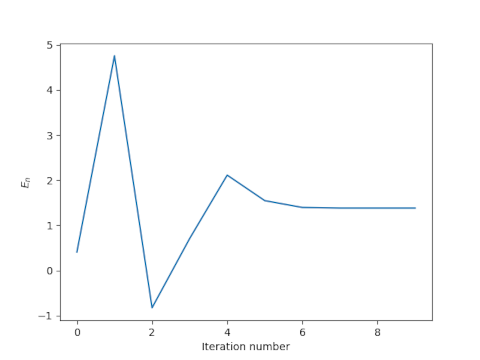
In this case Newton’s method converges to full floating point precision after a few iterations, but the road to convergence is rocky. After one iteration we have E = 5, even though we know a priori that E < π. Despite initially producing a nonsensical result, however, the method does converge.
The Ugly
The example above was taken from [1]. I wasn’t able to track down the original paper, but I saw it referenced second hand. The authors fixed M = 0.13π and let e = 0.991, 0.992, and 0.993. The results for e = 0.993 are similar to those for 0.991 above. But the authors reported that the method apparently doesn’t converge for e = 0.992. That is, the method works for two nearby values of e but not for a value in between.
Here’s what we get for the first few iterations.
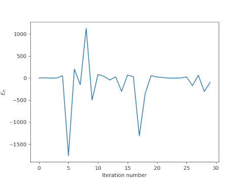
The method produces a couple spectacularly bad estimates for a solution known to be between 0 and π, and generally wanders around with no sign of convergence. If we look further out, it gets even worse.
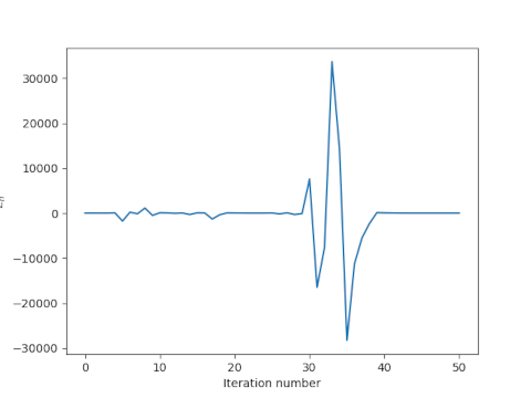
The previous bad iterates on the order of ±1000 pale in comparison to iterates roughly equal to ±30,000. Remarkably though, the method does eventually converge.
Commentary
The denominator in Newton’s method applied to Kepler’s equation is 1 – e cos E. When e is on the order of 0.99, this denominator can occasionally be on the order of 0.01, and dividing by such a small number can pull wild iterates closer to where they need to be. In this case Newton’s method is wandering around randomly, but if it ever wanders into a basin of attraction for the root, it will converge.
For practical purposes, if Newton’s method does not converge predictably then it doesn’t converge. You wouldn’t want to navigate a spacecraft using a method that in theory will eventually converge though you have no idea how long that might take. Still, it would be interesting to know whether there are any results that find points where Newton’s method applied to Kepler’s equation never converges even in theory.
The results here say more about Newton’s method and dynamical systems than about practical ways of solving Kepler’s equation. It’s been known for about three centuries that you can do better than always starting Newton’s method with E = M when solving Kepler’s equation.
[1] Charles, E. D. and Tatum, J.B. The convergence of Newton-Raphson iteration with Kepler’s Equation. Celestial Mechanics and Dynamical Astronomy. 69, 357–372 (1997).