Cologarithms and Entropy

Posted on 30 April 2021 by John

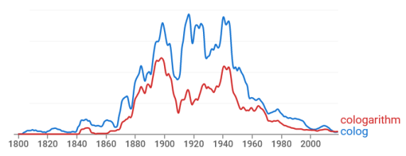
The term “cologarithm” was once commonly used but now has faded from memory. Here’s a plot of the frequency of the terms cololgarithm and colog from Google’s Ngram Viewer.

Frequency of colog and cologarithm

The cologarithm base b is the logarithm base 1/b, or equivalently, the negative of the logarithm base b.

colog_b x = log_1/b x = -log_b x

I suppose people spoke of cologarithms more often when they did calculations with logarithm tables.

Entropy

There’s one place where I would be tempted to use the colog notation, and that’s when speaking of Shannon entropy.

The Shannon entropy of a random variable with N possible values, each with probability p_i, is defined to be

$-\sum_{i=1}^N p_i \log_b \, p_i$

At first glace this looks wrong, as if entropy is negative. But you’re taking the logs of numbers less than 1, so the logs are negative, and the negative sign outside the sum makes everything positive.

If we write the same definition in terms of cologarithms, we have

$\sum_{i=1}^N p_i \,\text{colog}_b \, p_i$

which looks better, except it contains the unfamiliar colog.

Bits, nats, and dits

These days entropy is almost always measured in units of bits, i.e. using b = 2 in the definition above. This wasn’t always the case.

When logs are taken base e, the result is in units of nats. And when the logs are taken base 10, the result is in units of dits.

So binary logs give bits, natural logs give nats, and decimal logs give dits.

Bits are sometimes called “shannons” and dits were sometimes called “bans” or “hartleys.” The codebreakers at Bletchley Park during WWII used bans.

The unit “hartley” is named after Ralph Hartley. Hartley published a paper in 1928 defining what we now call Shannon entropy using logarithms base 10. Shannon cites Hartley in the opening paragraph of his famous paper A Mathematical Theory of Communication.

Chinese character frequency and entropy

Posted on 18 October 2019 by John

How much information is conveyed by a single Chinese character? This post addresses that question by computing Shannon entropy.

First of all, information theory defines the Shannon entropy of an “alphabet” to be

$-\sum_{i=1}^N p_i \log_2 p_i$

bits where p_i is the probability of the ith “letter” occurring and the sum is over all letters. I put alphabet and letter in quotes because information theory uses these terms for any collection of symbols. The collection could be a literal alphabet, like the Roman alphabet, or it could be something very different, such as a set of musical notes. For this post it will be a set of Chinese characters.

I’ll use a set of data on Chinese character frequency by Jun Da. See that site for details.

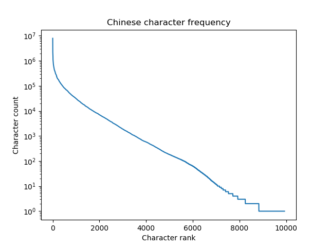
Here’s a plot of the character frequencies on a logarithmic scale.

Plotting Chinese character frequency, log scale

Jun Da’s data set contains 9,933 characters. The most common character, 的, appears 7,922,684 times in the language corpus and the least common character on the list, 鴒, appears once. The 1,000 most common characters account for 89% of use.

The Shannon entropy of the Chinese “alphabet” is 9.56 bits per character. By comparison, the entropy of the English alphabet is 3.9 bits per letter.

The entropy of individual symbols doesn’t tell the whole story of the information density of the two writing systems. Symbols are not independent, and so the information content of a sequence of symbols will be less than just multiplying the information content per symbol by the number of symbols. I imagine there is more sequential correlation between consecutive English letters than between consecutive Chinese characters, though I haven’t seen any data on that. If this is the case, just looking at the entropy of single characters underestimates the relative information density of Chinese writing.

Although writing vary substantially in how much information they convey per symbol, spoken languages may all convey about the same amount of information per unit of time.

A few weeks ago I wrote about new research suggesting that all human languages convey information at about the same rate. Some languages carry more information per syllable than others, as measured by Shannon entropy, but these languages are typically spoken more slowly. The net result is that people convey about 40 bits of information per second, independent of their language. Of course there are variations by region, by individual, etc. And there are limits to any study, though the study in question did consider a wide variety of languages.

Entropy extractor used in μRNG

Posted on 14 February 2019 by John

Yesterday I mentioned μRNG, a true random number generator (TRNG) that takes physical sources of randomness as input. These sources are independent but non-uniform. This post will present the entropy extractor μRNG uses to take non-uniform bits as input and produce uniform bits as output.

We will present Python code for playing with the entropy extractor. (μRNG is extremely efficient, but the Python code here is not; it’s just for illustration.) The code will show how to use the pyfinite library to do arithmetic over a finite field.

Entropy extractor

The μRNG generator starts with three bit streams—X, Y, and Z—each with at least 1/3 bit min-entropy per bit.

Min-entropy is Rényi entropy with α = ∞. For a Bernoulli random variable, that takes on two values, one with probability p and the other with probability 1-p, the min-entropy is

-log₂ max(p, 1-p).

So requiring min-entropy of at least 1/3 means the two probabilities are less than 2^-1/3 = 0.7937.

Take eight bits (one byte) at a time from X, Y, and Z, and interpret each byte as an element of the finite field with 2⁸ elements. Then compute

X*Y + Z

in this field. The resulting stream of bits will be independent and uniformly distributed, or very nearly so.

Purified noise

Just a quick aside. Normally you want to remove noise from data to reveal a signal. Said another way, you want to split the data into signal and noise so you can throw out the noise. Here the goal is the opposite: we want to remove any unwanted signal in order to create pure noise!

Python implementation

We will need the bernoulli class for generating our input bit streams, and the pyfinite for doing finite field arithmetic on the bits.

    from scipy.stats import bernoulli
    from pyfinite import ffield

And we will need a couple bit manipulation functions.

    def bits_to_num(a):
        "Convert an array of bits to an integer."
    
        x = 0
        for i in range(len(a)):
            x += a[i]*2**i
        return x

    def bitCount(n):
        "Count how many bits are set to 1."
        count = 0
        while(n):
            n &= n - 1
            count += 1
        return count

The following function generates random bytes using the entropy extractor. The input bit streams have p = 0.79, corresponding to min-entropy 0.34.

    def generate_byte():
        "Generate bytes using the entropy extractor."
    
        b = bernoulli(0.79)
    
        x = bits_to_num(b.rvs(8))
        y = bits_to_num(b.rvs(8))
        z = bits_to_num(b.rvs(8)) 

        F = ffield.FField(8)
        return F.Add(F.Multiply(x, y), z)

Note that 79% of the bits produced by the Bernoulli generator will be 1’s. But we can see that the output bytes are about half 1’s and half 0’s.

    s = 0
    N = 1000
    for _ in range(N):
        s += bitCount( generate_byte() )
    print( s/(8*N) )

This returned 0.50375 the first time I ran it and 0.49925 the second time.

For more details see the μRNG paper.

Update: RNG test suite results

I ran an experiment, creating streams of biased data and running them through the entropy extractor. The first post in the series, NIST STS, explains the set up. The last post in the series, using TestU01, summarizes the results. In a nutshell, the extractor passes STS and DIEHARDER, but fails PractRand and TestU01.

Solving for probability given entropy

Posted on 14 February 2019 by John

If a coin comes up heads with probability p and tails with probability 1-p, the entropy in the coin flip is

S = –p log₂ p – (1-p) log₂ (1-p).

It’s common to start with p and compute entropy, but recently I had to go the other way around: given entropy, solve for p. It’s easy to come up with an approximate solution.

entropy and approximation

Entropy in this case is approximately quadratic

S ≈ 4p(1-p)

and so

p ≈ (1 ± √(1-S))/2.

This is a good approximation if S is near 0 or 1 but mediocre in the middle. You could use solve for p numerically, say with Newton’s method, to get more accuracy if needed.

Update

As Sjoerd Visscher pointed out in the comments, the quadratic approximation for entropy is much better if you raise it to the power 3/4. When I added this new approximation to the graph above, the new approximation agreed with the correct value to within the thickness of the plotting line.

To make the approximation error visible, here’s the log of the absolute value of the error of the two approximations, on a log scale.

approximation error on log scale

The error in the new approximation is about an order of magnitude smaller, sometimes more.

The improved approximation for entropy is

S ≈ (4p(1-p))^3/4

and so the new approximation for probability is

p ≈ (1 ± √(1-S^4/3))/2.

Levenshtein distance from Finnegans Wake to Return of the Jedi

Posted on 21 November 2018 by John

Ewok

I ran into a delightfully strange blog post today called Finnegans Ewok that edits the first few paragraphs of Finnegans Wake to make it into something like Return of the Jedi.

(Unfortunately the page has gone away since I first wrote this. Some of the text is preserved in this Python script.)

The author, Adam Roberts, said via Twitter “What I found interesting here was how little I had to change Joyce’s original text. Tweak a couple of names and basically leave it otherwise as was.”

So what I wanted to do is quantify just how much had to change using the Levenshtein distance, which is essentially the number of one-character changes necessary to transform one string into another.

Here’s the first paragraph from James Joyce:

riverrun, past Eve and Adam’s, from swerve of shore to bend of bay, brings us by a commodius vicus of recirculation back to Howth Castle and Environs.

And here’s the first paragraph from Adam Roberts:

movierun, past new and hopes, from strike of back to bend of jeday, brings us by a commodius lucas of recirculation back to forestmoon and endor.

The original paragraph is 150 characters, the parody is 145 characters, and the Levenshtein distance is 44.

Here’s a summary of the results for the first four paragraphs.

    |-------+---------+----------|
    | Joyce | Roberts | Distance |
    |-------+---------+----------|
    |   150 |     145 |       44 |
    |   700 |     727 |      119 |
    |   594 |     615 |      145 |
    |  1053 |     986 |      333 |
    |-------+---------+----------|

The fifth paragraph seems to diverge more from Joyce. I maybe have gotten something misaligned, and reading enough of Finnegans Wake to debug the problem made my head hurt, so I stopped.

Update: See the next post for sequence alignment applied to the two sources. This lets you see not just the number of edits but what the edits are. This show why I was having difficulty aligning the fifth paragraphs.

Rényi Entropy

Posted on 21 November 2018 by John

Alfred Renyi

The most common way of measuring information is Shannon entropy, but there are others. Rényi entropy, developed by Hungarian mathematician Alfréd Rényi, generalizes Shannon entropy and includes other entropy measures as special cases.

Rényi entropy of order α

If a discrete random variable X has n possible values, where the ith outcome has probability p_i, then the Rényi entropy of order α is defined to be

$H_\alpha(X) = \frac{1}{1 - \alpha} \log_2 \left(\sum_{i=1}^n p_i^\alpha \right)$

for 0 ≤ α ≤ ∞. In the case α = 1 or ∞ this expression means the limit as α approaches 1 or ∞ respectively.

Rényi entropy of continuous random variable

The definition of Rényi entropy can be extended to continuous random variables by

$H_\alpha(X) = \frac{1}{1 - \alpha} \log_2 f_X(x)^\alpha \, dx$

but unlike the discrete case, Rényi entropy can be negative for continuous random variables, and so Rényi entropy is typically only used for discrete variables. For example, let X be the random variable defined on [1, ∞) with density

$f_X(x) = 3x^{-4}$

Then

$H_2(X) = - \int_1^\infty (3x^{-4})^2\, dx = -\log_2(9/7) = -0.36$

Special cases

Each value of α gives a possible entropy measure. All are additive for independent random variables. And for each discrete random variable X, H_α is a monotone non-decreasing function of α.

Max-entropy: α = 0

Assume all the probabilities p_i are positive. Then the H₀ is known as the max-entropy, or Hartley entropy. It is simply log₂n, the log of the number of values X takes on with positive probability.

Shannon entropy: α = 1

When α = 1 we get the more familiar Shannon entropy:

$H_1(X) = \lim_{\alpha\to1} H_\alpha(X) = - \left(\sum_{i=1}^n p_i \log_2 p_i \right)$

Collision entropy: α = 2

When the order α is not specified, it’s implicit default value is 2. That is, when people speak of Rényi entropy without qualification, they often have in mind the case α = 2. This case is also called collision entropy and is used in quantum information theory.

Min-entropy: α = ∞

In the limit as α goes to ∞, the Rényi entropy of X converges to the negative log of the probability of the most probable outcome. That is,

$H_{\infty}(X) = \lim_{\alpha\to\infty} H_\alpha(X) = - \log_2 \max p_i$

Relation to Lebesgue norms

Let p without a subscript be the vector of all the p_i. Then for α not equal to 1,

$H_\alpha(X) = \frac{\alpha}{1 - \alpha} \log_2 || p ||_\alpha$

As with Lebesgue norms, you use varying values of the parameter to emphasize various features.

Asymmetric surprise

Posted on 8 April 2018 by John

Motivating example: planet spacing

My previous post showed that planets are roughly evenly distributed on a log scale, not just in our solar system but also in extrasolar planetary systems. I hadn’t seen this before I stumbled on it by making some plots.

I didn’t think it was an original discovery—I assume someone did this exercise immediately when systems with several planets were discovered—but I didn’t know what this observation was called. I now know it’s known as the Titius-Bode law, a generalization of an observation about our solar system by Messrs. Titius and Bode a couple centuries ago. See, for example, [1].

Several people were skeptical of the claim that planets are distributed according to a power law and pointed out that uniformly distributed points can look fairly evenly distributed on a logarithmic scale. Which is true, and gets to the topic I want to discuss in this post. Planets are not spaced like uniform random samples (see [1]) and yet it reasonable, at first glance, to ask whether they are.

Asymmetric surprise

If you’re expecting a power law, and you’re given uniformly distributed data, it doesn’t look too surprising. On the other hand, if you’re expecting uniformly distributed data and you see data distributed according to a power law, you are surprised. I’ll formalize this below.

If you’ve ever tried to make a scaled model of our solar system, you were probably surprised that the planets are far from uniformly spaced. A scaled model of our solar system, say at a museum, is likely to position a few of the inner planets to scale, and then use text to explain where the outer planets should be. For example, there may be a footnote saying “And if everything were to scale, Pluto would be behind the Exxon station at the end of the street.” This is an example of implicitly expected a uniform distribution and receiving data distributed according to a power law.

Some people suspected that I was doing the opposite. By plotting distances on a log scale, I’m implicitly expected a power law distribution. Maybe the data were roughly uniform, but I fooled myself into seeing a power law.

Quantifying surprise

The Kullback-Leibler divergence from Y to X, written KL(X || Y), is the average surprise of seeing Y when you expected X. That’s one of the interpretations. See this post for more interpretations.

In general, Kullback-Leibler divergence is not symmetric. The divergence from X to Y typically does not equal the divergence from Y to X. The discussion above claims that the surprise from seeing power law data when expecting a uniform distribution is greater than the surprise from seeing uniform data when expected a power law distribution. We show below that this is true.

Let X be random variable uniformly distributed on [0, 1] and let Y be a random variable with distribution proportional to x^α on the same interval. (The proportionality constant necessary to make the probability integrate to 1 is α + 1.) We will show that KL(X || Y) is greater than KL(Y || X).

First we calculate the two divergences.

$\begin{eqnarray*} \mathrm{KL}(X || Y) &=& - \int_0^1 f_X(x) \, \log\left(\frac{f_Y(x)}{f_X(x)} \right) \, dx \\ &=& -\int_0^1 1 \cdot \left( \log(\alpha+1) + \alpha \log x - \log 1 \right) \, dx \\ &=& \alpha - \log(\alpha+1) \end{eqnarray*}$

and

$\begin{eqnarray*} \mathrm{KL}(Y || X) &=& - \int_0^1 f_Y(x) \, \log\left(\frac{f_X(x)}{f_Y(x)} \right) \, dx \\ &=& -\int_0^1 (\alpha + 1)x^\alpha \left(\log 1 -\log(\alpha+1) - \alpha \log x \right) \, dx \\ &=& \log(\alpha+1) - \frac{\alpha}{1 + \alpha} \end{eqnarray*}$

And here is a plot comparing the two results as a function of the exponent α.

***

[1] Timothy Bovaird, Charles H. Lineweaver; Exoplanet predictions based on the generalized Titius–Bode relation, Monthly Notices of the Royal Astronomical Society, Volume 435, Issue 2, 21 October 2013, Pages 1126–1138, https://doi.org/10.1093/mnras/stt1357

Bits of information in age, birthday, and birthdate

Posted on 2 March 2018 by John

birthday party

The previous post looked at how much information is contained in zip codes. This post will look at how much information is contained in someone’s age, birthday, and birth date. Combining zip code with birthdate will demonstrate the plausibility of Latanya Sweeney’s famous result [1] that 87% of the US population can be identified based on zip code, sex, and birth date.

Birthday

Birthday is the easiest. There is a small variation in the distribution of birthdays, but this doesn’t matter for our purposes. The amount of information in a birthday, to three significant figures, is 8.51 bits, whether you include or exclude leap days. You can assume all birthdays are equally common, or use actual demographic data. It only makes a difference in the 3rd decimal place.

Age

I’ll be using the following age distribution data found on Wikipedia.

|-----------+------------|
| Age range | Population |
|-----------+------------|
|  0– 4     |   20201362 |
|  5– 9     |   20348657 |
| 10–14     |   20677194 |
| 15–19     |   22040343 |
| 20–24     |   21585999 |
| 25–29     |   21101849 |
| 30–34     |   19962099 |
| 35–39     |   20179642 |
| 40–44     |   20890964 |
| 45–49     |   22708591 |
| 50–54     |   22298125 |
| 55–59     |   19664805 |
| 60–64     |   16817924 |
| 65–69     |   12435263 |
| 70–74     |    9278166 |
| 75–79     |    7317795 |
| 80–84     |    5743327 |
| 85+       |    5493433 |
|-----------+------------|

To get data for each particular age, I’ll assume ages are evenly distributed in each group, and I’ll assume the 85+ group consists of people from ages 85 to 92. [2]

With these assumptions, there are 6.4 bits of information in age. This seems plausible: if all ages were uniformly distributed between 0 and 63, there would be exactly 6 bits of information since 2⁶ = 64.

Birth date

If we assume birth days are uniformly distributed within each age, then age and birth date are independent. The information contained in the birth date would be the sum of the information contained in birthday and age, or 8.5 + 6.4 = 14.9 bits.

Zip code, sex, and age

The previous post showed there are 13.8 bits of information in a zip code. There are about an equal number of men and women, so sex adds 1 bit. So zip code, sex, and birth date would give a total of 29.7 bits. Since the US population is between 2²⁸ and 2²⁹, it’s plausible that we’d have enough information to identify everyone.

We’ve made a number of simplifying assumptions. We were a little fast and loose with age data, and we’ve assumed independence several times. We know that sex and age are not independent: more babies are boys, but women live longer. Still, Latanya Sweeney found empirically that you can identify 87% of Americans using the combination of zip code, sex, and birth date [1]. Her study was based on 1990 census data, and at that time the US population was a little less than 2²⁸.

Bits of information in a US zip code

Posted on 2 March 2018 by John

Mr. Zip

If you know someone’s US zip code, how much do you know about them? We can use entropy to measure the amount of information in bits.

To quantify the amount of information in a zip code, we need to know how many zip codes there are, and how evenly people are divided into zip codes.

There are about 43,000 zip codes in the US. The number fluctuates over time due to small adjustments.

Average information is maximized by dividing people into categories as evenly as possible. Maximum information about one person is maximized by dividing people into categories as unevenly as possible. To see this, suppose there were only two zip codes. The information we’d expect to learn from a zip code would be maximized if we divided people into two equal groups. Suppose on the other hand you were in one zip code and everyone else in the other. On average, zip code would reveal very little about someone, though it would reveal a lot about you!

If everyone were divided evenly into one of 43,000 zip codes, the amount of information revealed by knowing someone’s zip code would be about 15.4 bits, a little more information than asking 15 independent yes/no questions, each with equally likely answers.

But zip codes are not evenly populated. How much information is there in an actual five-digit zip code? To answer that question we need to know the population of each zip code. That’s a little tricky. Zip codes represent mail delivery points, not geographical areas. Technically the US Census Bureau tracks population by ZCTA (Zip Code Tabulation Area) rather than zip code per se. Population by ZCTA is freely available, but difficult to find. I gave up trying to find the data from official sources but was able to find it here.

We can go through the data and find the probability p of someone living in each ZCTA and add up –p log₂p over each area. When we do, we find that a ZTCA contains 13.83 bits of information. (We knew it had to be less than 15.4 because uneven distribution reduces entropy.)

The Safe Harbor provision of US HIPAA law lists zip codes as a quasi-identifier. Five digit zip codes do not fall under Safe Harbor. Three digit zip codes (the first three digits of five digit zip codes) do fall under Safe Harbor, mostly. Some areas are so sparsely populated that even three-digit zip code areas are considered too informative. Any three-digit zip code with fewer than 20,000 people is excluded. You can find a snapshot of the list here, though the list may change over time.

If we repeat our calculation for three-digit zip codes, we find that they carry about 9.17 bits of information. It makes little difference to the result whether you include sparse regions, exclude them, or lump them all into one region.

See the next post on information contained in age, birthday, and birth date.

Twenty questions and conditional probability

Posted on 16 November 2017 by John

The previous post compared bits of information to answers in a game of Twenty Questions.

The optimal strategy for playing Twenty Questions is for each question to split the remaining possibilities in half. There are a couple ways to justify this strategy: mixmax and average.

The minmax approach is to minimize the worse thing that could happen. The worst thing that could happen after asking a question is for your subject to be in the larger half of possibilities. For example, asking whether someone is left-handed is not a good strategy: the worst case scenario is “no,” in which case you’ve only narrowed your possibilities by 10%. The best mixmax approach is to split the population in half with each question.

The best average approach is also to split the possibilities in half each time. With the handedness example, you learn more if the answer is “yes,” but there’s only a 10% change that the answer is yes. There’s a 10% chance of gaining 3.322 bits of information, but a 90% chance of only gaining 0.152 bits. So the expected number of bits, the entropy, is 0.469 bits. Entropy is maximized when all outcomes are equally likely. That means you can’t learn more than 1 bit of information on average from a yes/no question, and you learn the most when both possibilities are equally likely.

Now suppose you want to ask about height and sex. As in the previous post, we assume men and women’s heights are normally distributed with means 70 and 64 inches respectively, and both have standard deviation 3 inches.

If you ask whether a person is taller than 67 inches, you split a mixed population of men and women in half. You will learn 1 bit of information from this question, but you’ve put yourself in a suboptimal position for the next question. A height of at least 67 inches half of the adult population in general, but it selects a majority of men and a minority of women. And as we discussed above, uneven splits are suboptimal, in the worst case and on average.

If you’re going to ask about height and sex, ask about sex first. If the person is female, ask next whether her height is above 64 inches. But if the person is male, ask whether his height is above 70 inches. That is, you want to split the population evenly at each step conditioning on your previous answer. A cutoff of 67 inches is optimal unconditionally, but suboptimal if you condition on sex.

The optimal strategy for Twenty Questions is to ask a question with probability of 1/2 being true, conditional on all previous data. You might get lucky with uneven conditional splits, but on average, and in the worst case, you won’t do as well.

Entropy

Bits, nats, and dits

Related posts

Related linguistic posts

Entropy extractor

Purified noise

Python implementation

Update: RNG test suite results

Related posts

Update

More information theory posts

Related posts

Rényi entropy of order α

Rényi entropy of continuous random variable

Special cases

Max-entropy: α = 0

Shannon entropy: α = 1

Collision entropy: α = 2

Min-entropy: α = ∞

Relation to Lebesgue norms

More information theory posts

Motivating example: planet spacing

Asymmetric surprise

Quantifying surprise

Related posts

Birthday

Age

Birth date

Zip code, sex, and age

More privacy posts

Related privacy posts