Riff on an integration bee integral

Posted on 16 May 2025 by John

I saw an integral posted online that came from this year’s MIT Integration Bee.

$\int_0^1 x^{2024} (1 - x^{2025})^{2025}\, dx$

My thoughts on seeing this were, in order:

It looks like a beta function.
The answer is a small number.
You can evaluate the integral using the substitution u = 1 − x²⁰²⁵.

I imagine most students’ reactions would be roughly the opposite. They’d first see the substitution. Some might think of the value being small, and none would think of beta functions.

Size estimate

The value of the integral is small because you have numbers between 0 and 1 being raised to large powers. In real applications, being able to estimate the size of integral may be more valuable than being able to compute the integral.

But on a quiz, like the Integration Bee, knowing that the result is small would be worthless, except possibly to check a result. You know from the context of the problem being on a timed quiz that there must be a trick [1].

Incidentally, if you changed the problem slightly, say by replacing one of the instances of 2025 with 2025.03, the integration problem becomes much harder, but you could still estimate that the value is small.

Beta functions

The first time I saw someone evaluate an integral by recognizing a beta function it seemed like he was pulling a rabbit out of a hat. I was completely surprised that he thought something was common knowledge that I’d never seen.

Years later I went to work in biostatistics at MDACC and worked with the beta function and beta random variables all the time. If you look through my publications, you’ll see the word “beta” appears several times.

The beta function is defined as follows. You could take the first equality as the definition and the second as a theorem.

$B(x, y) = \int_0^1 t^{x-1} (1 - t)^{y-1} \,dx = \frac{\Gamma(x) \, \Gamma(y)}{\Gamma(x+y)}$

The integrand in the definition of the beta function is the probability density function for a beta(x, y) random variable, and so B(x, y) is the normalizing constant for a beta(x, y) probability distribution.

The integral in the Integration Bee question is not a beta function. I thought maybe it could be turned into a beta function, but the u substitution is simpler.

If you change the integrand above to

$\int_0^1 x^{2024} (1 - x)^{2025}\, dx$

then you do have a beta function. The value of this integral is B(2025, 2026) which equals 2024! 2025! / 4050!, which is an extremely small number.

Numerical estimation

The integral in the previous section is roughly the same as that of x²⁰²⁴ (1 − x)²⁰²⁴. This function has its maximum at ½, and so the integrand is less than 2⁻⁴⁰⁴⁸ ≈ 10⁻¹²¹⁹.

If we want to evaluate 2024! 2025! / 4050! numerically we’ll need to be indirect about it because 2024! would overflow and the final result would underflow. We could calculate the log base 10 of the value using Python as follows.

>>> from scipy.special import gammaln
>>> from math import log
>>> (gammaln(2025) + gammaln(2026) - gammaln(4051))/log(10)
-1220.576093208249

So our upper bound got us to within an order of magnitude or two of the result.

[1] When you see the current year used in a math problem, the quiz writer is winking at you. The year is often meant to suggest that a number is large but somewhat arbitrary. Here you suspect that the key to the question would be the same if 2024 and 2025 were replaced with 1997 and 1998. Also, the year is often a hint that you don’t want to use brute force. In this case, it’s a warning not to expand the integrand using the binomial theorem.

Logarithmic sawtooth

Posted on 12 April 2025 by John

Here’s a strange integral I ran across recently [1].

$\int_0^1 \log(x) \bmod 2 = \frac{1}{\tanh(1)}$

It’s a little surprising that the integral even exists, and more surprising that its value has a simple expression.

Here’s a plot of the integrand.

The plot doesn’t do justice to all the activity on the left end. There are an infinite number of increasingly vertical segments piled up on the left end as x goes to 0.

If you were to plot the integrand on a log scale, you’d get a sawtooth wave, stretching back to negative infinity.

I would expect the integral to be difficult to evaluate numerically without some special handling, but SciPy’s quod function does a decent job by default.

    from numpy import log, tanh
    from scipy.integrate import quad

    print(quad(lambda x: log(x)%2, 0, 1))
    print(1/tanh(1))

This evaluates the integral as 1.313042… while the exact value is 1.313035…

To the integrator’s credit, it warns of difficulties before producing the result:

IntegrationWarning: The maximum number of subdivisions (50) has been achieved.

If increasing the limit yields no improvement it is advised to analyze the integrand in order to determine the difficulties. If the position of a local difficulty can be determined (singularity, discontinuity) one will probably gain from splitting up the interval and calling the integrator on the subranges. Perhaps a special-purpose integrator should be used.

[1] Matthew A. Niemiro. The Natural Logarithm Modulo 2. The American Mathematical Monthly, Vol. 128, No. 2 (FEBRUARY 2021), p. 177.

A better integral for the normal distribution

Posted on 31 August 2024 by John

For a standard normal random variable Z, the probability that Z exceeds some cutoff z is given by

$\mbox{Prob}(Z \geq z) = Q(z) = \frac{1}{\sqrt{2\pi}} \int_z^\infty \exp(-x^2/2)\, dx$

If you wanted to compute this probability numerically, you could obviously evaluate its defining integral numerically. But as is often the case in numerical analysis, the most obvious approach is not the best approach. The range of integration is unbounded and it varies with the argument.

J. W. Craig [1] came up with a better integral representation, better from the perspective of numerical integration. The integration is always over the same finite interval, with the argument appearing inside the integrand. The integrand is smooth and bounded, well suited to numerical integration.

For positive z, Craig’s integer representation is

$Q(z) = \frac{1}{\pi} \int_0^{\pi/2} \exp\left( -\frac{z^2}{2\sin^2 \theta} \right) \, d\theta$

Illustration

To show that the Craig’s integral is easy to integrate numerically, we’ll evaluate it using Gaussian quadrature with only 10 integration points.

    from numpy import sin, exp, pi
    from scipy import integrate
    from scipy.stats import norm

    for x in [0.5, 2, 5]:
        q, _ = integrate.fixed_quad(
            lambda t: exp(-x**2 / (2*sin(t)**2))/pi,
            0.0, pi/2, n=10)
        print(q, norm.sf(x))

(SciPy uses sf (“survival function”) for the CCDF. More on that here.)

The code above produces the following.

    0.30858301 0.30853754
    0.02274966 0.02275013
    2.86638437e-07 2.86651572e-07

So with 10 integration points, we get four correct figures. And the accuracy seems to be consistent for small, medium, and large values of x. (Five standard deviations is pretty far out in the tail of a normal distribution, as evidenced by the small value of the integral.)

[1] J. W. Craig, A new, simple and exact result for calculating the probability of error for two-dimensional signal constellations, in TEEE MILCOM’91 Conf. Rec., Boston, MA (1991) рр. 25.2.1-25.5.5.

MCMC and the coupon collector problem

Posted on 6 May 2024 by John

Bob Carpenter wrote today about how Markov chains cannot thoroughly cover high-dimensional spaces, and that they do not need to. That’s kinda the point of Monte Carlo integration. If you want systematic coverage, you can/must sample systematically, and that’s impractical in high dimensions.

Bob gives the example that if you want to get one integration point in each quadrant of a 20-dimensional space, you need a million samples. (2²⁰ to be precise.) But you may be able to get sufficiently accurate results with a lot less than a million samples.

If you wanted to be certain to have one sample in each quadrant, you could sample at (±1, ±1, ±1, …, ±1). But if for some weird reason you wanted to sample randomly and hit each quadrant, you have a coupon collector problem. The expected number of samples to hit each of N cells with uniform [1] random sampling with replacement is

N( log(N) + γ )

where γ is Euler’s constant. So if N = 2²⁰, the expected number of draws would be over 15 million.

[1] We’re assuming each cell is sampled independently with equal probability each time. Markov chain Monte Carlo is more complicated than that because the draws are not independent.

The Borwein integrals

Posted on 13 February 2024 by John

The Borwein integrals introduced in [1] are a famous example of how proof-by-example can go wrong.

Define sinc(x) as sin(x)/x. Then the following equations hold.

$\begin{align*} \int_0^\infty \text{sinc}(x) \,dx &= \frac{\pi}{2} \\ \int_0^\infty \text{sinc}(x) \, \text{sinc}\left(\frac{x}{3}\right) \,dx &= \frac{\pi}{2} \\ \int_0^\infty \text{sinc}(x)\, \text{sinc}\left(\frac{x}{3}\right) \,\text{sinc}\left(\frac{x}{5}\right) \,dx &= \frac{\pi}{2} \\ \vdots &\phantom{=} \\ \int_0^\infty \text{sinc}(x) \, \text{sinc}\left(\frac{x}{3}\right) \cdots \text{sinc}\left(\frac{x}{13}\right) \,dx &= \frac{\pi}{2} \\ \end{align*}$

However

$\int_0^\infty \text{sinc}(x) \, \text{sinc}\left(\frac{x}{3}\right) \cdots \text{sinc}\left(\frac{x}{15}\right) \,dx = \frac{\pi}{2} - \delta$

where δ ≈ 2.3 × 10⁻¹¹.

This is where many presentations end, concluding with the moral that a pattern can hold for a while and then stop. But I’d like to go just a little further.

Define

$B(n) = \int_0^\infty \prod_{k=0}^{n} \text{sinc}\left(\frac{x}{2k+1}\right) \, dx.$

Then B(n) = π/2 for n = 1, 2, 3, …, 6 but not for n = 7, though it almost holds for n = 7. What happens for larger values of n?

The Borwein brothers proved that B(n) is a monotone function of n, and the limit as n → ∞ exists. In fact the limit is approximately π/2 − 0.0000352.

So while it would be wrong to conclude that B(n) = π/2 based on calculations for n ≤ 6, this conjecture would be approximately correct, never off by more than 0.0000352.

[1] David Borwein and Jonathan Borwein. Some Remarkable Properties of Sinc and Related Integrals. The Ramanujan Journal, 3, 73–89, 2001.

Integrals involving secants and tangents

Posted on 18 December 2023 by John

As a student, I often made the mistake of thinking that if I knew a more powerful theorem, I didn’t need to learn a less powerful theorem. The reason this is a mistake is that the more powerful theorem may be better by one obvious criterion but not be better by other less-obvious criteria.

The most powerful solution technique is not always the best, not because there’s anything immoral about using an over-powered technique, but because the most powerful technique in theory might not be that useful in practice.

The most powerful technique for integrating rational functions of trig functions is Weierstrass’ t = tan(x/2) trick which I wrote about a few days ago. In principle, Weierstrass’ trick reduces integrating any rational combination of trig functions to integrating a rational function of x. And in principle, partial factions reduce any such integral to closed form.

But that which is doable in principle may not be doable in practice. If it is doable, this might not be the easiest approach.

If P is a polynomial in two variables, then [1] proves that

$\int P(\sec x, \tan x) \, \sec x\, dx = F(u) - G(v) + c \log u + C$

where

$\begin{align*} u &= \sec x + \tan x \\ v &= \sec x - \tan x \\ \end{align*}$

If your integral has the form above, this approach will probably be far simpler than using Weierstrass’ substitution.

The key to proving the theorem above is to use the facts

$\begin{align*} \sec x &= \frac{u+v}{2} \\ \tan x &= \frac{u-v}{2} \\ uv &= 1 \end{align*}$

You can find a detailed explanation in [1], but essentially the equations above are enough to not only prove the theorem but to compute F and G.

The paper gives an example, integrating

$\int 16 \sec^5 x\, dx$

in less than half a printed page. Computing the integral with Weierstrass’ trick would require integrating

$\int 32 \frac{(1 + t^2)^4}{(1 - t^2)^5} \, dt$

which must be possible, though it seems daunting.

Incidentally, the paper also shows how to compute integrals of the form

$\int P(\sec x, \tan x) \, dx$

removing the requirement of a factor of sec x outside the polynomial.

[1] Jonathan P. McCammond. Integrating Polynomials in Secant and Tangent. The American Mathematical Monthly, Nov., 1999, Vol. 106, No. 9, pp. 856–858

The world’s sneakiest substitution

Posted on 7 December 2023 by John

Something that seems like an isolated trick may turn out to be much more important. This is the case with a change of variables discovered by Karl Weierstrass.

Every calculus student learns a handful of standard techniques: u-substitutions, partial fractions, integration by parts, and trig substitutions. Then there is one more technique that is like something off a secret menu, something know only to the cognoscenti: Weierstrass’ t = tan(x/2) trick [1]. Michael Spivak called this “the world’s sneakiest substitution.”

The world's sneakiest substitution is undoubtedly t = tan(x/2), x = 2 arctan t, dx = 2 dt / (1 + t^2)

This was on page 325 of the first edition of Spivak’s Calculus, page 360 of the second edition.

This innocent but apparently unmotivated change of variables has the following magical consequences:

sin(x) = 2t/(1 + t²)
cos(x) = (1 – t²) / (1 + t²)
dx = 2 dt/(1 + t²).

This means that the trick can convert an integral containing any rational combination of trig functions into one involving only rational functions, which then can (in principle) be integrated in closed form using partial fractions. It’s the key that unlocks all trig integrals.

However, this is not as practical as it sounds. You may get a high-degree rational function, and while in theory the rational function can be integrated using partial fractions, the decomposition may be tedious if not impossible. Still, it’s interesting that a single trick reduces one large class of integration problems to another.

Now let’s leave integration behind. The equations above say that as t varies, the functions 2t/(1 + t²) and (1 – t²) / (1 + t²) take on all the values that sin(x) and cos(x) do. This means, for example, that you can draw a circle using graphics hardware that does not support sines and cosines. In theory the range of t would have to be infinite, but in practice the range would only have to be large enough to fill in the right pixels.

If we can parameterize a circle with rational functions, what else can we parameterize this way? It turns out, for example, that elliptic curves do not have rational parameterizations. This question is its own niche of algebraic geometry. I don’t know the history here, but it’s plausible some of this math was motivated by wondering what else could be done along the lines of Weierstrass’ trick.

[1] When I’ve mentioned this trick before, some have told me this was a routine part of their course. That was not my experience, either as a student or as an instructor. As a freshman I learned the trick from a friend who was the best of our cohort at integration, someone who would have done well at an integration bee if we’d had one. I felt I’d been let in on a secret.

Numerical integral with a singularity

Posted on 26 November 2023 by John

Richard Hamming [1] gives this nice example of an integral with a mild singularity:

$\int_0^1 \log(\sin(x))\, dx$

The integrand approaches −∞ as x approaches 0 and yet the integral is finite. If we try into numerically evaluate this integral, we will either get inaccurate results or we will have to go to a lot of work.

This post will show that with a clever reformulation of the problem we use simple methods to get accurate results, or use sophisticated methods with fewer function evaluations.

As I wrote about years ago, a common technique for dealing with singularities is to add and subtract a function with the same asymptotic behavior that can be integrated by hand. Hamming does a slight variation on this, multiplying and dividing by x inside the logarithm.

$\begin{align*} \int_0^1 \log(\sin(x))\, dx &= \int_0^1 \log(x)\, dx + \int_0^1 \log\left(\frac{\sin(x)}{x}\right) \, dx \\ &= -1 + \int_0^1 \log\left(\frac{\sin(x)}{x}\right) \, dx \end{align*}$

Here we integrated the singular part, log(x), and we are left with numerically integrating a well-behaved function, one that is smooth and bounded on the interval of integration. Because sin(x) ≈ x for small x, we can define sin(x)/x to be 1 at 0 and have a smooth function.

We’ll use NumPy’s sinc function to handle sin(x)/x properly near 0. There are two conventions for defining the sinc function, either as sin(x)/x or as sin(πx)/πx. NumPy uses the latter convention, so we define our own sinc function as follows.

import numpy as np
def mysinc(x): return np.sinc(x/np.pi)

Trapezoid rule

Let’s use the simplest numerical method, the trapezoid rule.

We run into a problem immediately: if we chop up the interval [0, 1] in a way that puts an integration point at 0, our resulting integral will be infinite. We could replace 0 with some ε > 0, but if we do, we should try a few different values of ε to see whether our choice of ε greatly impacts our integral.

for ε in [1e-6, 1e-7, 1e-8]:
    xs = np.linspace(ε, 1, 100)
    integral = sum( np.log(np.sin(x)) for x in xs ) / 100

This gives us

-1.152996659484881
-1.1760261818509377
-1.1990523999312201

suggesting that the integral does indeed depend on ε. We’ll see soon that our integral evaluates to around −1.05. So our results are not accurate, and the smaller ε is, the worse our answer is. [2]

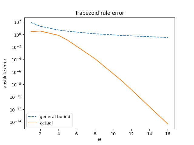
Now let’s evaluate the integral as Hamming suggests. We’ll use a varying number of integration points so the difference between our integral estimates will give us some idea whether we’re converging.

for N in [25, 50, 100]:
    xs = np.linspace(0, 1, N)
    integral = sum( np.log(mysinc(xs)) )/N
    integral -= 1 # subtract the integral of log(x)
    print(integral)

This gives us

-1.0579531812873197
-1.057324013010989
-1.057019035348765

The consistency between the result suggests the integral is around −1.057.

Adaptive integration

We said at the top of this article that Hamming’s reformulation would either let us get accurate results from simple methods or let us get by with fewer function evaluations using a sophisticated method. Now we’ll demonstrate the latter, using the adaptive integration algorithm quad from SciPy.

from scipy.integrate import quad

# Integrate log(sin(x)) from 0 to 1
integral, error = quad(lambda x: np.log(np.sin(x)), 0, 1)
print(integral, error) 

# Integrate log(x sin(x)/x) = log(x) + log(mysinc(x)) from 0 to 1
integral, error = quad(lambda x: np.log(mysinc(x)), 0, 1)
integral -= 1
print(integral, error)

This prints

-1.0567202059915843 1.7763568394002505e-15
-1.056720205991585 6.297207865333937e-16

suggesting that both approaches are working. Both estimate their error to be near machine precision. But as we’ll see, the direct approach uses about 10 times as many function evaluations.

Let’s ask quad to return more details by adding full_output = 1 as an argument.

integral, error, info = quad(lambda x: np.log(np.sin(x)), 0, 1, full_output=1)
print(integral, error, info["neval"])

integral, error, info = quad(lambda x: np.log(mysinc(x)), 0, 1, full_output=1)
integral -= 1
print(integral, error, info["neval"])

This shows that the first integration used 231 function evaluations, but the second used only 21.

The difference in efficiency doesn’t matter when you’re evaluating an integral one time, but if you were repeatedly evaluating similar integrals inside a loop, subtracting off the singularity could make your problem run 10 times faster. Simulations involving Bayesian statistics can have such integrations in the inner loop, and so making an integration an order of magnitude faster could make the overall simulation an order of magnitude faster, reducing CPU-days to CPU-hours.

[1] Richard Hamming, Numerical Methods for Scientists and Engineers. Second edition. Dover.

[2] We can get better results if we let ε and 1/N go to zero at the same rate. The following code produces mediocre results, but better results than above.

for N in [10, 100, 1000]:
    xs = np.linspace(1/N, 1, N)
    integral = sum( np.log(np.sin(x)) for x in xs ) / N
    print(integral)

This prints

-0.8577924592777062
-1.0253626377143321
-1.05243363818431

which at least seems to be getting closer to the correct result, but has bad accuracy for so many function evaluations.

Regular solids and Monte Carlo integration

Posted on 29 September 2023 by John

Monte Carlo integration is not as simple in practice as it is often introduced. A homework problem might as you to integrate a function of two variables by selecting random points from a cube and counting how many of the points fall below the graph of the function. This would indeed give you an estimate of the volume bounded by the surface and hence the value of the integral.

But Monte Carlo integration is most often used in high dimensions, and the region of interest takes up a tiny proportion of a bounding box. In practice you’d rarely sample uniformly from a high-dimensional box. This post will look at sampling points on a (possibly high-dimensional) sphere.

The rate of convergence of Monte Carlo integration depends on the variance of the samples, and so people look for ways to reduce variance. Antipodal sampling is one such approach. The idea is that a function on a sphere is likely to take on larger values on one side of the sphere and smaller values on the other. So for every point x where the function is sampled, it is also sampled at the diametrically opposite point −x on the assumption/hope that the values of the function at the two points are negatively correlated.

Antipodal sampling is a first step in the direction of a hybrid of regular and random sampling, sampling by random choices of regularly spaced points, such as antipodal points. When this works well, you get a sort of synergy, an integration method that converges faster than either purely systematic or purely random sampling.

If a little is good, then more is better, right? Not necessarily, but maybe, so it’s worth exploring. If I remember correctly, Alan Genz explored this. Instead of just taking antipodal points, you could sample at the points of a regular solid, like a tetrahedron. Randomly select and initial point, create a tetrahedron on the sphere with this as one of the vertices, and sample your integrand at each of the vertices. Or you could think of having a tetrahedron fixed in space and randomly rotating the sphere so that the sphere remains in contact with the vertices of the tetrahedron.

If you’re going to sample at the vertices of a regular solid, you’d like to know what regular solids are possible. In three dimensions, there are five: tetrahedron, hexahedron (cube), octahedron, dodecahedon, and icosahedron. Only the first three of these generalize to dimensions 5 and higher, so you only have three choices in high dimension if you want to sample at the vertices of a regular solid.

Here’s more about the cross polytope, the generalization of the octahedron.

If you want more regularly-spaced points on a sphere than regular solids will permit, you could compromise and use points whose spacing is approximately regular, such as the Fibonacci lattice. You could randomly rotate your Fibonacci lattice to create a randomized quasi-Monte Carlo (RQMC) method.

You have a knob you can turn determining the amount of regularity and the amount of randomness. At one extreme is purely random sampling. As you turn the knob you go from antipodes to tetrahedra and up to cross polytopes. Then there’s a warning line, but you can keep going with things like the Fibonacci lattice, introducing some distortion, sorta like turning the volume of a speaker up past the point of distortion.

In my experience, I’ve gotten the best results near the random sampling end of the spectrum. Antipodal sampling sped up convergence, but other methods not so much. But your mileage may vary; the results depend on the kind of function you’re integrating.

Quadrature rules and an impossibility theorem

Posted on 25 August 2023 by John

Many numerical integration formulas over a finite interval have the form

$\int_a^b f(x)\, dx = \sum_{i=1}^n w_i\, f(x_i) + C f^{(k)}(\xi)$

That is, the integral on the left can be approximated by evaluating the integrand f at particular nodes and taking the weighted sum, and the error is some multiple of a derivative of f evaluated at a point in the interval [a, b].

This post will give several examples, showing how they all fit into to framework above, then discuss the impossibility of extending this framework to infinite integrals.

Simpson’s 3/8 rule

Simpson’s rule says

$\int_{x_0}^{x_3} f(x) \, dx = \frac{3h}{8} \Big(f(x_0) + 3f(x_1) + 3f(x_2) + f(x_3) \Big)- \frac{3f^{(4)}(\xi) h^5}{80}$

In this case the x‘s are evenly spaced a distance of h apart. The weights are 3h/8, 9h/8, 9h/8, and 3h/8.

We have n = 4, k = 4, and C = −3h^5/80.

We don’t know a priori what the value of ξ will be, only that there will be some value of ξ between x₀ and x₃ that makes the equation hold. If we have an explicit bound on the 4th derivative of f then we have an explicit bound on the error in approximating the integral by the weighted sum.

Bode’s rules

A sequence of quadrature rules go by the name “Bode’s rule.” Here is one example, also known as Weddle’s rule.

$\begin{align*} \int_{x_0}^{x_6} f(x)\, dx = \frac{h}{140}&\Big(41 f(x_0) + 216f(x_1) + 27 f(x_2) +272 f(x_3) \\ &+ 27 f(x_4) + 216 f(x_5) + 41 f(x_6) \Big) \\ &-\frac{9 f^{(8)}(\xi) h^9}{1400} \end{align}$

As with Simpson’s 3/8 rule, you could map the formula for Bode’s rule(s) to the template at the top of the post.

Gauss quadrature

Gauss’ formula says

$\int_{-1}^1 f(x)\, dx = \sum_{i=1}^n w_i\, f(x_i) + C f^{(2n)}(\xi)$

for some ξ in [−1, 1]. Here the limits of integration are fixed, though you could use a change of variables to integrals over other finite integrals into this form.

Unlike Bode’s rule and Simpson’s rule, the x‘s are not evenly spaced but are the zeros of P_n, the Legendre polynomial of degree n. The weights are related to the x‘s and the derivative P′_n evaluated at the x‘s. The constant C is a complicated function of n but is independent of f.

Note that the error term involves the (2n)th derivative of f. This explains why Gaussian integration can be more accurate than other methods using the same number of function evaluations. The non-uniform spacing of the integration nodes enables higher-order error terms.

Non-existence theorem

Although many integration rules over a finite interval have the form

$\int_a^b f(x)\, dx = \sum_{i=1}^n w_i\, f(x_i) + C f^{(k)}(\xi)$

Davis and Rabinowitz [1] proved that there cannot be an integration rule of the form

$\int_0^\infty f(x)\, dx = \sum_{i=1}^n w_i\, f(x_i) + C f^{(k)}(\xi)$

The proof, given in [1], takes only about one page. The entire article is a little more than a page, and about half the article is preamble to the proof.

[1] P. J. Davis and P. Rabinowitz. On the Nonexistence of Simplex Integration Rules for Infinite Integrals. Mathematics of Computation, Vol. 26, No. 119 (July, 1972), pp. 687–688

Integration

Riff on an integration bee integral

Size estimate

Beta functions

Numerical estimation

Logarithmic sawtooth

Related posts

A better integral for the normal distribution

Illustration

Related posts

MCMC and the coupon collector problem

Related posts

The Borwein integrals

Integrals involving secants and tangents

Related posts

The world’s sneakiest substitution

Numerical integral with a singularity

Trapezoid rule

Adaptive integration

Related posts

Regular solids and Monte Carlo integration

Quadrature rules and an impossibility theorem

Simpson’s 3/8 rule

Bode’s rules

Gauss quadrature

Non-existence theorem

Related posts