Long permutations and long cycles

A permutation rearranges the elements of a list. The number of arrangements, say of a deck of cards, is finite, so eventually you have to arrive at an arrangement you’ve produced before, and history will repeat itself. Along the way, some cards may move in smaller cycles than others.

Example

For example, consider the permutation

p = [5, 6, 2, 1, 0, 8, 3, 4, 9, 7]

that sends i to p(i). Here indices start with 0.

The number 2 is a fixed point: p(2) = 2. So it has a cycle length of 1.

The number 1 is part of a cycle of length 3: p(1) = 6, p(6) = 3, and p(3) = 1.

The longest cycle is [0, 5, 8, 9, 7, 4] which has length 6.

Longest cycles

What happens to the length of cycles as you permute longer lists? Obviously the longest possible cycle increases with the length of the list, but what happens to the average length of the longest cycle?

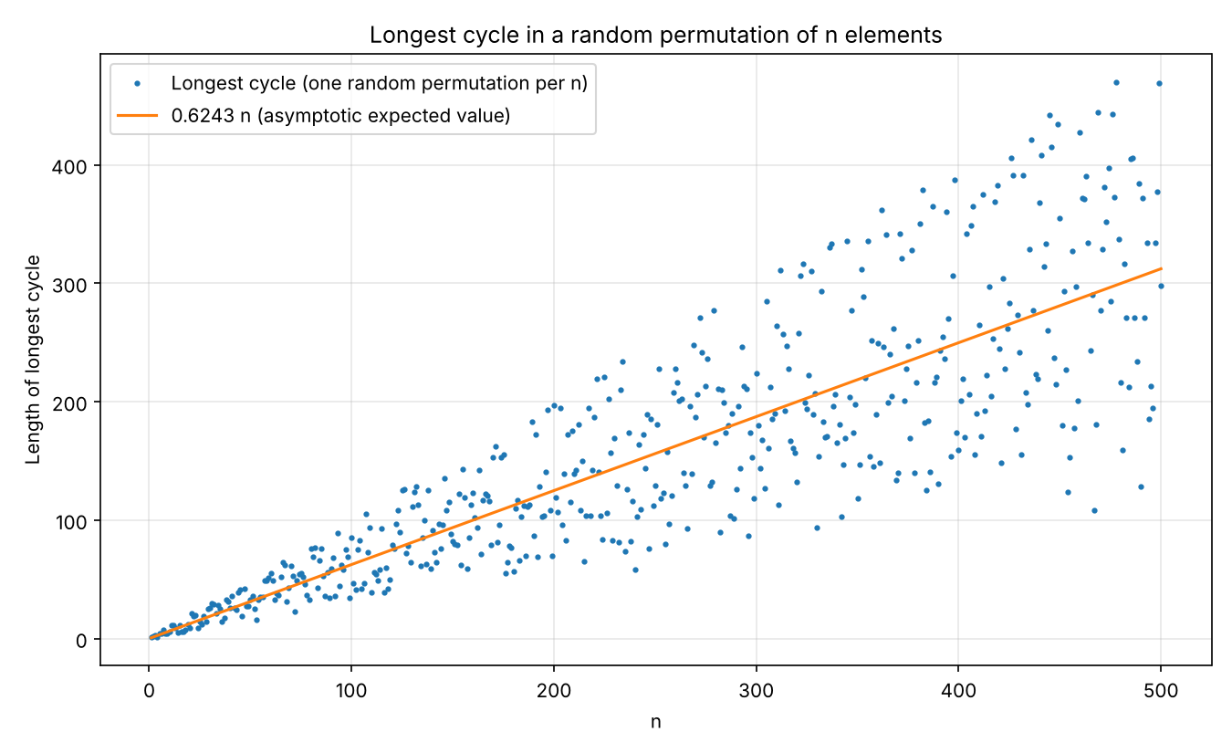
Let Ln be the length of the longest cycle in a random permutation of n items. You’d expect the average value of Ln, written E[Ln], would increase when n increases. But do they increase at the same rate? Conceivably E[Ln] goes to infinity as n goes to infinity, but at a slower rate, say proportional to √n rather than proportional to n. Let’s make a plot to see.

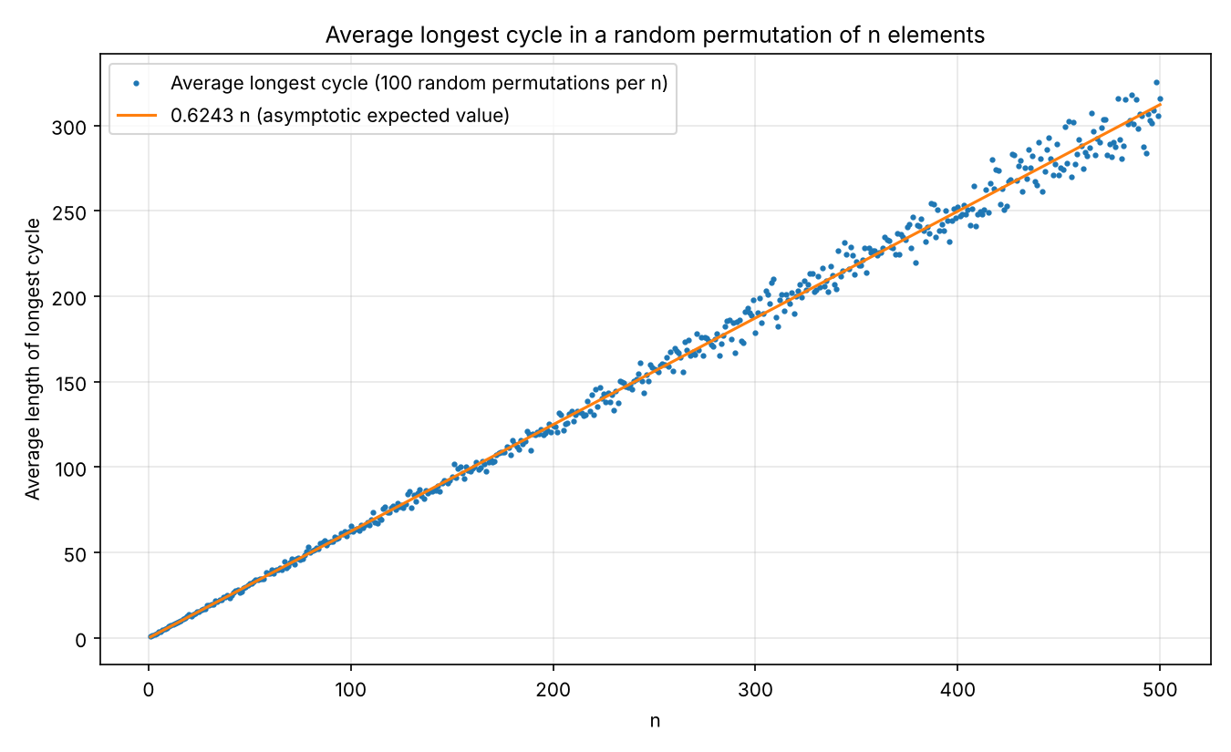
There’s a lot of variance, but the central tendency looks approximately linear in n. Let’s repeat our experiment, this time creating 100 random permutations of each size and averaging their maximum cycle lengths.

As we’d expect from the central limit theorem, averaging over 100 samples reduced the scatter by about a factor of 10.

It appears that the expected value of the maximum cycle length grows in proportion to n, and in fact the expected value is somewhere around 0.6n. In the example at the top of the post, the longest cycle is exactly 0.6n. I didn’t plan that: the permutation example was chosen at random.

Asymptotic value

The limit of the ratio E[Ln]/n is known to be

\lim_{n\to\infty} \frac{\text{E}[L_n]}{n} = \int_0^1 \exp(\text{li}(t)) \, dt = 0.6243\ldots

Shepp and Lloyd [1] proved the result above. The constant on the right hand side is known as the Golomb-Dickman constant. I think Golomb investigated E[Ln]/n and had found that there was a limiting value, but Shepp and Lloyd were the first to give a closed-form expression for the limit. Dickman had run into the same constant in a theorem in number theory.

[1] L. A. Shepp and S. P. Lloyd, “Ordered Cycle Lengths in a Random Permutation,” Transactions of the American Mathematical Society, vol. 121, no. 2, pp. 340–357, February 1966.

Fraction comparison trick revisited

A few years ago I wrote about a curious result: a/b is usually greater than c/d when a + d is greater than b + c. And “usually” means with probability 11/12.

As stated in the post, you can make this statement rigorous by choosing integers up to size N at random and taking the limit as N goes to infinity.

We can also choose a, b, c, and d uniformly from [0, 1]. This is similar to choosing four integers up to N and dividing all the integers by N, which doesn’t change the probabilities.

Now a/b > c/d if and only if ad > bc, so another way to state the theorem is that

Prob(ad > bc | a + d > b + c) = 11/12.

Or to state it yet another way, pick two pairs of numbers at random. The probability that the pair with the larger sum also has the larger product is 11/12. That seems more intuitive to me than the original statement.

If a + d is greater than b + c, it’s likely that a/b is greater than c/d. It seems plausible that if a + d is much greater than b + c, it’s more likely that a/b is greater than c/d. Or in terms of cross products, the more the sum of one pair is bigger than the sum of the other, the more likely the product of the former is to be greater than the latter. That is

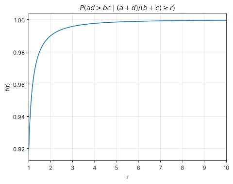
f(r) = Prob(ad > bc | (a + d)/(b + c) ≥ r)

should be an increasing function of r. We know the probability above equals 11/12 when r = 1. We expect that the probability should approach 1 as r goes to infinity.

This is indeed the case, as shown in the plot below.

In particular, f(2) ≈ 0.99 and f(6) ≈ 0.999. So if a + d is two (or six) times bigger than b + c, there is a 0.99 (or 0.999) probability that ad is larger than bc.

You can calculate f(r) analytically or estimate it by simulation. I had Claude do both and they produce comparable results. There is a closed-form expression for f(r) but it’s really complicated.

The von Mises-Fisher distribution

Probability density function must integrate to 1, and so if you know a density function up to a constant, the constant is determined.

When you’re looking at a probability density f(x) for the first time, it helps to ignore the normalizing constant. Concentrate on the part of the function involving x and know that the normalizing constant is whatever it has to be. For example, about half of the ink that it takes to write down a beta or chi-squared density is devoted to the normalization constant; the rest of the expression is easier to understand.

This post will do the opposite of the advice above and focus on normalization constants because this ties into the previous post on modified Bessel functions.

The von Mises probability distribution on a circle has two parameters, μ and κ, and its density function is

f(x \mid \mu, \kappa) = \frac{\exp(\kappa \cos(x - \mu))}{2\pi I_0(\kappa)}

The normalizing constant is 2π I0(κ). The factor of 2π is unsurprising for anything defined on a circle. The more interesting part is I0, the modified Bessel function of order 0.

The von Mises-Fisher distribution is the generalization of the von Mises distribution to a sphere in p dimensions. The density function is

f(\mathbf{x} \mid \boldsymbol{\mu}, \kappa) = C_{p}(\kappa) \exp \left( {\kappa \boldsymbol{\mu}^\mathsf{T} \mathbf{x} } \right)

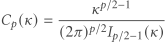
where the normalization constant Cp(κ) is

C_{p}(\kappa)=\frac {\kappa^{p/2-1}} {(2\pi)^{p/2}I_{p/2-1}(\kappa)}

where Ip/2 − 1 is the modified Bessel function of order p/2 − 1. The values of x and μ are in bold face because they are now vectors, points on the unit sphere.

When p = 2, we have the “sphere” in two dimensions, i.e. the circle, and the von Mises-Fisher distribution reduces to the von Mises distribution. But where did the cosine go? The inner product of x and μ is the cosine of the angle between the two vectors.

When p = 3, obviously an important special case, the von Mises-Fisher distribution is known as the Fisher distribution. In that case the normalizing constant C3(κ) can be written without using modified Bessel functions because when ν = ½ + n for an integer n, Iν(x) is an elementary function.

Calculating the expected range of normal samples

The previous post looked at the expected IQ range in a jury of 12. This post will look more generally at computing the expected range of n samples from a N(0, 1) random variable. This will give the expected range in units of σ, i.e. multiply the results by σ if your σ isn’t 1.

As mentioned in the previous post, the expected range is given by

d_n = 2n \int_{-\infty}^\infty \Phi(x)^{n-1} \, x\,\phi(x) \, dx

where φ and Φ are the PDF and CDF of a standard normal. The integral can be calculated in closed form for n ≤ 5, but in general it requires numerical integration [1].

The following Python code can compute dn.

from scipy.stats import norm
from scipy.integrate import quad
import numpy as np

def d(n):
    integrand = lambda x: x*norm.pdf(x)*norm.cdf(x)**(n-1)
    res, info = quad(integrand, -np.inf, np.inf)
    return 2*n*res

For large n we have the asymptotic approximation

d_n = 2 \Phi^{-1}\left( \frac{n \,–\, 0.375}{ n + 0.25} \right)

which we could implement in Python by

def approx(n):
    return 2*norm.ppf((n - 0.375)/(n + 0.25))

For very large n the asymptotic expression may be more accurate than the integral due to numerical integration error.

Here are a few example values.

|-----+-------|
|   n |   d_n |
|-----+-------|
|   2 | 1.128 |
|   3 | 1.693 |
|   5 | 2.326 |
|  10 | 3.078 |
|  12 | 3.258 |
|  23 | 3.858 |
|  50 | 4.498 |
| 100 | 5.015 |
|-----+-------|

[1] Order Statistics by H. A. David. John Wiley & Sons. 1970.

Expected IQ spread on a jury

There’s been some discussion online lately about how a large difference in IQ makes it difficult for two people to communicate. There have been studies that confirm this effect. The difficulty is not insurmountable, but it takes deliberate effort to overcome.

Someone dismissed this communication difficulty by pointing out that the expected difference in IQ between two individuals is around 17, suggesting that most communication is between people who differ by more than one standard deviation in IQ. But this calculation assumes people are chosen at random, which they usually are not. People tend to live around and work around others of similar intelligence.

However, a jury is a random sample. It’s not a perfect random sample. For one thing, it starts with a random sample of people who are registered to vote, or who have a driver’s license, not all individuals. Furthermore, the pool of potential jurors is reduced to a jury through the process of voir dire, which is not random.

For this post I will make the simplifying assumption that a jury is a random sample from a population with normally distributed IQ with standard deviation σ = 15. The mean doesn’t matter here, but you could assume it’s 100 if you’d like.

By symmetry, the expected range of n samples from a normal random variable is twice the maximum. For n = 12 the range is about 3.26σ, which corresponds to nearly 50 IQ points.

This suggests there’s usually a big spread of IQ on a jury. Even if IQ doesn’t measure intelligence, it measures something, and that something varies a lot over 12 people chosen at random [1].

Related posts

[1] In case you’re interested in the technical details, the expected range of n samples from a standard normal random variable is given by

d_n = 2n \int_{-\infty}^\infty \Phi(x)^{n-1} \, x\,\phi(x) \, dx

where φ and Φ are the PDF and CDF of a standard normal. Multiply this by σ to get the range of a normal random variable with standard deviation σ. As for how to calculate dn, see the next post.

Probability that a random binary matrix is invertible

The two latest posts have involved invertible matrices with 0 and 1 entries. If you fill an n × n matrix with 0s and 1s randomly, how likely is it to be invertible?

What kind of inverse?

There are a couple ways to find the probability that a binary matrix is invertible, depending on what you mean by the inverse.

Suppose you have a matrix M filled with 0s and 1s and you’re looking for a matrix N such that MN is the identity matrix. Do you want the entries of N to also be 0s and 1s? And when you multiply the matrices, are you doing ordinary integer arithmetic or are you working mod 2?

In the previous posts we were working over GF(2), the field with two elements, 0 and 1. All the elements of a matrix are either 0 or 1, and arithmetic is carried out mod 2. In that context there’s a nice expression for the probability a square matrix is invertible.

If you’re working over the real numbers, the probability of binary matrix being invertible is higher. One way to see this is that the inverse of a binary matrix is allowed to be binary but it isn’t required to be.

Another way to see this is to look at determinants. If you think of a matrix M as a real matrix whose entries happen to only be 0 or 1, M is invertible if and only its determinant is non-zero. But if you think of M as a matrix over GF(2), the entries are either 0 or 1 out of necessity, and M is invertible if and only if its determinant, computed in GF(2), is non-zero. If the determinant of M as a real matrix is a non-zero even number, then M is invertible as a real matrix but not as a matrix over GF(2).

Probability of invertibility in GF(2)

Working over GF(2), what is the probability that a random matrix is invertible? Turns out it’s just as easy to answer a more general question: what is the probability that a random n × n matrix over GF(q), a finite field with q elements, is invertible? This is

\prod_{i=1}^n\left( 1 - \frac{1}{q^i} \right)

When q = 2 and n = 8 this probability is 0.289919. The probability is roughly the same for all larger values of n, converging to approximately 0.288788 as n → ∞.

Probability of invertibility in ℝ

What is the probability that an 8 × 8 matrix with random 0 and 1 entries is invertible as a real matrix? We can estimate this by simulation.

import numpy as np

def simulate_prob_invertible_real(n, numreps=1000):
    s = 0
    for _ in range(numreps):
        M = np.random.randint(0, 2, size=(n, n))
        det = np.linalg.det(M)
        if abs(det) > 1e-9:
            s += 1
    return s/numreps

When n = 8, I got 0.5477 when running the code with 10,000 reps.

When n = 32, I got a probability of 1. Obviously it is possible for a 32 × 32 binary matrix to be singular, but it’s very unlikely: it didn’t happen in 10,000 random draws.

Random samples from a tetrahedron

Exactly one month ago I wrote about sampling points from a triangle. This post will look at the three dimensional analog, sampling from a tetrahedron. The generalization to higher dimensions works as well.

Sampling from a triangle

In the triangle post, I showed that a naive approach doesn’t work but a variation does. If the vertices of the triangle are A, B, and C, then the naive approach is to generate three uniform random numbers, normalize them, and use them to form a linear combination of the vertices. That is, generate

r1, r2, r3

uniformly from [0, 1], then define

r1′ = r1/(r1 + r2 + r3)
r2′ = r2/(r1 + r2 + r3)
r3′ = r3/(r1 + r2 + r3)

and return as a random sample the point

r1′ A + r2′ B + r3′ C.

This oversamples points near the middle of the triangle and undersamples points near the vertices. But everything above works if you replace uniform samples with exponential samples.

Sampling from a tetrahedron

The analogous method works for a tetrahedron with vertices A, B, C, and D. Generate exponential random variables ri for i = 1, 2, 3, 4. Then normalize, defining each ri′ to be ri divided by the sum of all the ri s. Then the random sample is

r1′ A + r2′ B + r3′ C + r4′ D.

In the case of the triangle, it was easy to visualize that uniformly generated rs did not lead to uniform samples of the triangle, but that exponentially generated rs did. This is harder to do in three dimensions. Even if the points were uniformly sampled from a tetrahedron, they might not look uniformly distributed from a given perspective.

So how might we demonstrate that our method works? One approach would be to take a cube inside a tetrahedron and show that the proportion of samples that land inside the cube is what we’d expect, namely the ratio of the volume of the cube to the volume of the tetrahedron.

This brings up a couple interesting subproblems.

  1. How do we compute the volume of a tetrahedron?
  2. How can we test whether our cube lies entirely within the tetrahedron?

Volume of a tetrahedron

To find the volume of a tetrahedron, form a matrix M whose columns are the vectors from three of the vertices to the remaining vertex. So we could take A − D, B − D, and C − D. The volume of the tetrahedron is the determinant of M divided by 6.

Testing whether a cube is inside a tetrahedron

A tetrahedron is convex, and so the line segment joining any two points inside the tetrahedron lies entirely inside the tetrahedron. It follows that if all the vertices of a cube are inside the a tetrahedron, the entire cube is inside.

So this brings us to the problem of testing whether a point is inside a tetrahedron. We can do this by converting the coordinates of the point to barycentric coordinates, then testing whether all the coordinates are non-negative and add to 1.

Random sampling illustration

I made up four points as vertices of a tetrahedron.

import numpy as np

A = [0, 0, 0]
B = [5, 0, 0]
C = [0, 7, 0]
D = [0, 1, 6]
A, B, C, D = map(np.array, [A, B, C, D])

For my test cube I chose the cube whose vertex coordinates are all combinations of 1 and 2. So the vertex nearest the origin is (1, 1, 1) and the vertex furthest from the origin is (2, 2, 2). You can verify that all the vertices are inside the tetrahedron, and so the cube is inside the tetrahedron.

The tetrahedron has volume 35, and the cube has volume 1, so we expect 1/35th of the random points to land inside the cube. Here’s the code to sample the tetrahedron and calculate the proportion of points that land in the cube.

from scipy.stats import expon

def incube(v):
    return 1 <= v[0] <= 2 and 1 <= v[1] <= 2 and 1 <= v[2] <= 2

def good_sample(A, B, C, D):
    r = expon.rvs(size=4)
    r /= sum(r)
    return r[0]*A + r[1]*B + r[2]*C + r[3]*D

def bad_sample(A, B, C, D):
    r = np.random.random(size=4)
    r /= sum(r)
    return r[0]*A + r[1]*B + r[2]*C + r[3]*D

N = 1_000_000

badcount  = 0
goodcount = 0

for _ in range(N):
    v = bad_sample(A, B, C, D)
    if incube(v):
        badcount += 1        
    v = good_sample(A, B, C, D)
    if incube(v):
        goodcount += 1

print(badcount/N, goodcount/N, 1/35)

This produced

0.094388 0.028372 0.028571…

The good (exponential) method match the expected proportion to three decimal places but the bad (uniform) method put about 3.3 times as many points in the cube as expected.

Note that three decimal agreement is about what we’d expect via the central limit theorem since 1/√N = 0.001.

If you’re porting the sampler above to an environment where you don’t a function for generating exponential random samples, you can roll your own by returning −log(u) where u is a uniform sample from [0. 1].

More general 3D regions

After writing the post about sampling from triangles, I wrote a followup post about sampling from polygons. In a nutshell, divide your polygon into triangles, then randomly select a triangle in proportion to its area, then sample with that triangle. You can do the analogous process in three dimensions by dividing a general volume into tetrahedra.

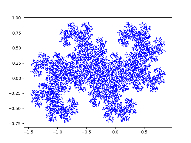
Randomly generated dragon

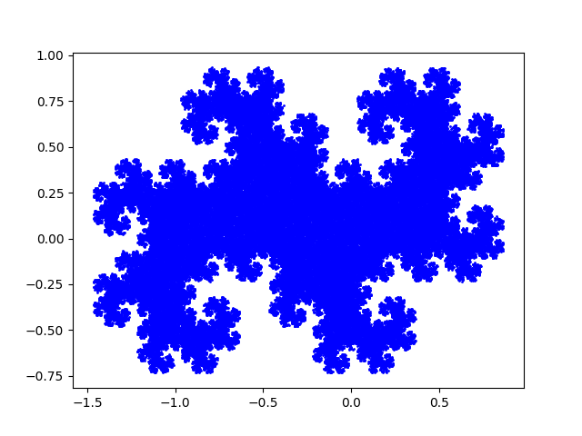
Here’s a simple way to generate a fractal known as the Twin Dragon. Start with random values of x and y and repeatedly update the according to the rule

xnew = (− xold + yold)/2 − b
ynew = (− xold − yold)/2

where b is randomly chosen to be 0 or 1 with equal probability. The plot of these points fills in the Twin Dragon.

Here’s what the plot looks like after 10,000 iterations.

And after 100,000 iterations.

Here’s the Python script I used to make the plots.

import matplotlib.pyplot as plt
from numpy.random import random, choice

x, y = random(), random()
for _ in range(100000):
    x, y = (-x + y)/2, (-x - y)/2
    x -= choice([0, 1])
    plt.plot(x, y, 'bo', markersize=1)
plt.show()

The algorithm used here is a particularly special case of a more general algorithm for generating similar fractals found in [1].

Update: Here’s a different way to produce the same fractal from Donald Knuth.

Here’s a similar post from several years ago:
The chaos game and the Sierpinski triangle

[1] Darst, Palagallo, and Price. Fractal Tilings in the Plane. Mathematics Magazine [71]:1, 1998.

1000 most common words

Last week I wrote about a hypothetical radio station that plays the top 100 songs in some genre, with songs being chosen randomly according to Zipf’s law. The nth most popular song is played with probability proportional to 1/n.

This post is a variation on that post looking at text consisting of the the 1,000 most common words in a language, where word frequencies follow Zipf’s law.

How many words of text would you expect to read until you’ve seen all 1000 words at least once? The math is the same as in the radio station post. The simulation code is the same too: I just changed a parameter from 100 to 1,000.

The result of a thousand simulation runs was an average of 41,246 words with a standard deviation of 8,417.

This has pedagogical implications. Say you were learning a foreign language by studying naturally occurring text with a relatively small vocabulary, such as newspaper articles. You might have to read a lot of text before you’ve seen all of the thousand most common words.

On the one hand, it’s satisfying to read natural text. And it’s good to have the most common words reinforced the most. But it might be more effective to have slightly engineered text, text that has been subtly edited to make sure common words have not been left out. Ideally this would be done with such a light touch that it isn’t noticeable, unlike heavy-handed textbook dialogs.

Simple error function approximation

I recently ran across the fact that

\int_0^x \exp(-t^2)\, dt \approx \sin(\sin(x))

is a remarkably good approximation for −1 ≤ x ≤ 1.

Since the integral above defines the error function erf(x), modulo a constant, this says we have a good approximation for the error function

\text{erf}(x) \approx \frac{2}{\sqrt{\pi}} \sin( \sin(x) )

again provided −1 ≤ x ≤ 1.

The error function is closely related to the Gaussian integral, i.e. the normal probability distribution CDF Φ. The relation between erf and Φ is simple but error-prone. I wrote up some a page notes for myself a few years ago so I wouldn’t make a mistake again moving between these functions and their inverses.

Update: This post makes the connection to probability explicit.

You can derive the approximation by writing out the power series for exp(t), substituting −t² for t, and integrating term-by-term from 0 to x. You’ll see that the result is the same as the power series for sine until you get to the x5 term, so the error is on the order of x5. Here’s a plot of the error.

The error is extremely small near 0, which is what you’d expect since the error is on the order of x5.