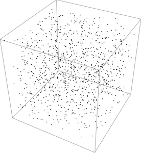
Regular solids and Monte Carlo integration

Posted on 29 September 2023 by John

Monte Carlo integration is not as simple in practice as it is often introduced. A homework problem might as you to integrate a function of two variables by selecting random points from a cube and counting how many of the points fall below the graph of the function. This would indeed give you an estimate of the volume bounded by the surface and hence the value of the integral.

But Monte Carlo integration is most often used in high dimensions, and the region of interest takes up a tiny proportion of a bounding box. In practice you’d rarely sample uniformly from a high-dimensional box. This post will look at sampling points on a (possibly high-dimensional) sphere.

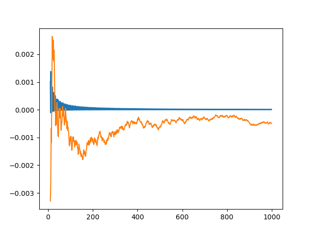
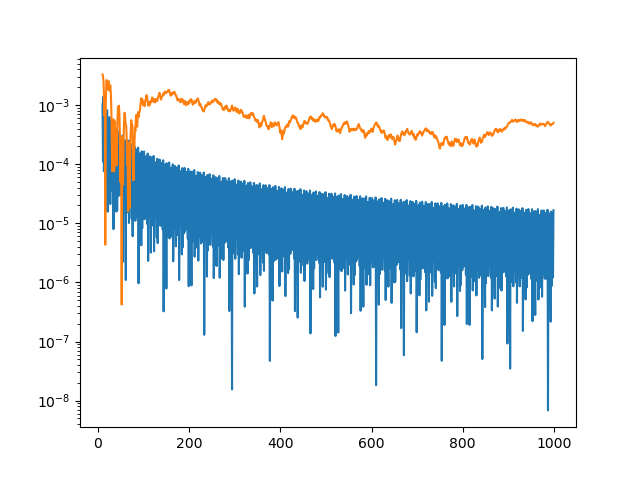
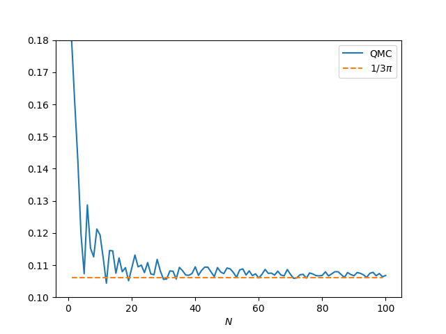
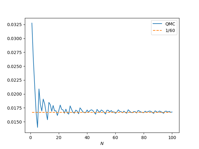
The rate of convergence of Monte Carlo integration depends on the variance of the samples, and so people look for ways to reduce variance. Antipodal sampling is one such approach. The idea is that a function on a sphere is likely to take on larger values on one side of the sphere and smaller values on the other. So for every point x where the function is sampled, it is also sampled at the diametrically opposite point −x on the assumption/hope that the values of the function at the two points are negatively correlated.

Antipodal sampling is a first step in the direction of a hybrid of regular and random sampling, sampling by random choices of regularly spaced points, such as antipodal points. When this works well, you get a sort of synergy, an integration method that converges faster than either purely systematic or purely random sampling.

If a little is good, then more is better, right? Not necessarily, but maybe, so it’s worth exploring. If I remember correctly, Alan Genz explored this. Instead of just taking antipodal points, you could sample at the points of a regular solid, like a tetrahedron. Randomly select and initial point, create a tetrahedron on the sphere with this as one of the vertices, and sample your integrand at each of the vertices. Or you could think of having a tetrahedron fixed in space and randomly rotating the sphere so that the sphere remains in contact with the vertices of the tetrahedron.

If you’re going to sample at the vertices of a regular solid, you’d like to know what regular solids are possible. In three dimensions, there are five: tetrahedron, hexahedron (cube), octahedron, dodecahedron, and icosahedron. Only the first three of these generalize to dimensions 5 and higher, so you only have three choices in high dimension if you want to sample at the vertices of a regular solid.

Here’s more about the cross polytope, the generalization of the octahedron.

If you want more regularly-spaced points on a sphere than regular solids will permit, you could compromise and use points whose spacing is approximately regular, such as the Fibonacci lattice. You could randomly rotate your Fibonacci lattice to create a randomized quasi-Monte Carlo (RQMC) method.

You have a knob you can turn determining the amount of regularity and the amount of randomness. At one extreme is purely random sampling. As you turn the knob you go from antipodes to tetrahedra and up to cross polytopes. Then there’s a warning line, but you can keep going with things like the Fibonacci lattice, introducing some distortion, sorta like turning the volume of a speaker up past the point of distortion.

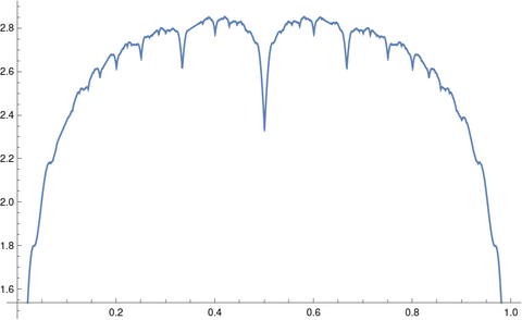
In my experience, I’ve gotten the best results near the random sampling end of the spectrum. Antipodal sampling sped up convergence, but other methods not so much. But your mileage may vary; the results depend on the kind of function you’re integrating.

Quadrature rules and an impossibility theorem

Posted on 25 August 2023 by John

Many numerical integration formulas over a finite interval have the form

$\int_a^b f(x)\, dx = \sum_{i=1}^n w_i\, f(x_i) + C f^{(k)}(\xi)$

That is, the integral on the left can be approximated by evaluating the integrand f at particular nodes and taking the weighted sum, and the error is some multiple of a derivative of f evaluated at a point in the interval [a, b].

This post will give several examples, showing how they all fit into to framework above, then discuss the impossibility of extending this framework to infinite integrals.

Simpson’s 3/8 rule

Simpson’s rule says

$\int_{x_0}^{x_3} f(x) \, dx = \frac{3h}{8} \Big(f(x_0) + 3f(x_1) + 3f(x_2) + f(x_3) \Big)- \frac{3f^{(4)}(\xi) h^5}{80}$

In this case the x‘s are evenly spaced a distance of h apart. The weights are 3h/8, 9h/8, 9h/8, and 3h/8.

We have n = 4, k = 4, and C = −3h^5/80.

We don’t know a priori what the value of ξ will be, only that there will be some value of ξ between x₀ and x₃ that makes the equation hold. If we have an explicit bound on the 4th derivative of f then we have an explicit bound on the error in approximating the integral by the weighted sum.

Boole’s rules

A sequence of quadrature rules go by the name “Boole’s rule.” Here is one example, also known as Weddle’s rule.

$\begin{align*} \int_{x_0}^{x_6} f(x)\, dx = \frac{h}{140}&\Big(41 f(x_0) + 216f(x_1) + 27 f(x_2) +272 f(x_3) \\ &+ 27 f(x_4) + 216 f(x_5) + 41 f(x_6) \Big) \\ &-\frac{9 f^{(8)}(\xi) h^9}{1400} \end{align}$

As with Simpson’s 3/8 rule, you could map the formula for Boole’s rule(s) to the template at the top of the post.

Gauss quadrature

Gauss’ formula says

$\int_{-1}^1 f(x)\, dx = \sum_{i=1}^n w_i\, f(x_i) + C f^{(2n)}(\xi)$

for some ξ in [−1, 1]. Here the limits of integration are fixed, though you could use a change of variables to integrals over other finite integrals into this form.

Unlike Bode’s rule and Simpson’s rule, the x‘s are not evenly spaced but are the zeros of P_n, the Legendre polynomial of degree n. The weights are related to the x‘s and the derivative P′_n evaluated at the x‘s. The constant C is a complicated function of n but is independent of f.

Note that the error term involves the (2n)th derivative of f. This explains why Gaussian integration can be more accurate than other methods using the same number of function evaluations. The non-uniform spacing of the integration nodes enables higher-order error terms.

Non-existence theorem

Although many integration rules over a finite interval have the form

$\int_a^b f(x)\, dx = \sum_{i=1}^n w_i\, f(x_i) + C f^{(k)}(\xi)$

Davis and Rabinowitz [1] proved that there cannot be an integration rule of the form

$\int_0^\infty f(x)\, dx = \sum_{i=1}^n w_i\, f(x_i) + C f^{(k)}(\xi)$

The proof, given in [1], takes only about one page. The entire article is a little more than a page, and about half the article is preamble to the proof.

[1] P. J. Davis and P. Rabinowitz. On the Nonexistence of Simplex Integration Rules for Infinite Integrals. Mathematics of Computation, Vol. 26, No. 119 (July, 1972), pp. 687–688

Pushing numerical integration software to its limits

Posted on 12 June 2023 by John

The previous post discussed the functions

$f_n(x) = \sum_{k=1}^n \frac{|\sin( k\pi x )|}{k}$

as test cases for plotting. This post will look at using the same functions as test cases for integration. As you can see from the plot of f₃₀(x) below, the function is continuous, but the derivative of the function has a lot of discontinuities.

The integrals of Steinerberger’s functions can be computed easily in closed form. Each term in the sum integrates to 2/πk and so

$\int_0^1 f_n(x)\, dx = \frac{2}{\pi} \sum_{k=1}^n \frac{1}{k} = 2 H_n / \pi$

where H_n is the nth harmonic number.

Symbolic integration

When I tried to get Mathematica to compute the integral above for general n it got stuck.

When I tried the specific case of 10 with

    Integrate[f[x, 10], {x, 0, 1}]

it churned for a while, then returned a complicated expression involving nested radicals:

    (1/(79380 \[Pi]))(465003 + 400 Sqrt[2 (48425 - 13051 Sqrt[5])] -
    35600 Sqrt[2 (5 - Sqrt[5])] + 42800 Sqrt[2 (5 + Sqrt[5])] -
    400 Sqrt[2 (48425 + 13051 Sqrt[5])])

Mathematica could not simplify the result to

    HarmonicNumber[10] 2/Pi]

but it could confirm that the two expressions are numerically equal within the limitations of floating point precision.

Assuming the two expressions for the integral are equal, it would be interesting to see why this is so. I don’t see off hand where the radicals above come from.

Numerical integration

When I asked Mathematica to compute the integral above numerically with

    NIntegrate[f[x, 10], {x, 0, 1}]

it produced an answer which correct to four decimal places and a warning

NIntegrate failed to converge to prescribed accuracy after 9 recursive bisections in x near {x} = {0.667953}. NIntegrate obtained 1.8646445043323603` and 2.908590085997311`*^-6 for the integral and error estimates.

Even though NIntegrate didn’t achieve full precision, it warned that this was the case. It produced a decent answer and a fairly good estimate of its error, about half of the actual error.

I tried numerically integrating the same function with Python.

    from scipy.integrate import quad
    quad(lambda x: f(x, 10), 0, 1)

Python’s quad function did about the same as Mathematica’s NIntegrate. It produced the following warning:

IntegrationWarning: The maximum number of subdivisions (50) has been achieved. If increasing the limit yields no improvement it is advised to analyze the integrand in order to determine the difficulties. If the position of a local difficulty can be determined (singularity, discontinuity) one will probably gain from splitting up the interval and calling the integrator on the subranges. Perhaps a special-purpose integrator should be used. (1.8646395747766926, 0.0024098799348653954)

This error message is more helpful, and the error estimate 0.0024 is an upper bound on the error.

Increasing the number of subdivisions by a factor of 10 with

    quad(lambda x: f(x, 10), 0, 1, limit=500)

eliminated the warning and made the integration much more accurate.

Expected distance between points in a cube

Posted on 6 May 2023 by John

random samples from a cube

Suppose you randomly sample points from a unit cube. How far apart are pairs of points on average?

My intuition would say that the expected distance either has a simple closed form or no closed form at all. To my surprise, the result is somewhere in between: a complicated closed form.

Computing the expected value by simulation is straight forward. I’ll make the code a little less straight forward but more interesting and more compact by leveraging a couple features of NumPy.

    import numpy as np

    dimension = 3
    reps = 10000

    cube1 = np.random.random((reps, dimension))
    cube2 = np.random.random((reps, dimension))
    distances = np.linalg.norm(cube1 - cube2, axis=1)
    print(distances.mean())

This gives a value of 0.6629. This value is probably correct to two decimal places since the Central Limit Theorem says our error should be on the order of one over the square root of the number of reps.

In fact, the expected value given here is

$\frac{4}{105} + \frac{17}{105}\sqrt{2} - \frac{2}{35}\sqrt{3} + \frac{1}{5}\log(1 + \sqrt{2}) + \frac{2}{5}\log(2 + \sqrt{3}) - \frac{1}{15}\pi$

which evaluates numerically to 0.661707….

The expression for the expected value is simpler in lower dimensions; it’s just 1/3 in one dimension. In higher dimensions there is no closed form in terms of elementary functions and integers.

Incidentally, the image above was made using the following Mathematica code.

    pts = RandomPoint[Cube[], 10^3];
    Graphics3D[{PointSize[Small], Point[pts], Opacity[0.3]}, Boxed -> True]

Golden integration

Posted on 29 April 2023 by John

Let φ be the golden ratio. The fractional parts of nφ bounce around in the unit interval in a sort of random way. Technically, the sequence is quasi-random.

Quasi-random sequences are like random sequences but better in the sense that they explore a space more efficiently than random sequences. For this reason, Monte Carlo integration (“integration by darts“) can often be made more efficient by replacing random sequences with quasi-random sequence. This post will illustrate this efficiency advantage in one dimension using the fractional parts of nφ.

Here are functions that will generate our integration points.

    from numpy import random, zeros

    def golden_source(n):
        phi = (1 + 5**0.5)/2
        return (phi*n)%1

    def random_source(N):
        return random.random()

We will pass both of these generators as arguments to the following function which saves a running average of function evaluates at the generated points.

    def integrator(f, source, N):
        runs = zeros(N)
        runs[0] = f(source(0))
        for n in range(1, N):
            runs[n] = runs[n-1] + (f(source(n)) - runs[n-1])/n
        return runs

We’ll use as our example integrand f(x) = x² (1 − x)³. The integral of this function over the unit interval is 1/60.

    def f(x):
        return x**2 * (1-x)**3
    exact = 1/60

Now we call our integrator.

    random.seed(20230429)
    N = 1000
    golden_run = integrator(f, golden_source, N)
    random_run = integrator(f, random_source, N)

Now we plot the difference between each run and the exact value of the integral. Both methods start out with wild fluctuations. We leave out the first 10 elements in order to make the error easier to see.

    import matplotlib.pyplot as plt

    k = 10
    x = range(N)
    plt.plot(x[k:], golden_run[k:] - exact)
    plt.plot(x[k:], random_run[k:] - exact)

This produces the following plot.

The integration error using φn − ⌊φn⌋ is so close to zero that it’s hard to observe its progress. So we plot it again, this time taking the absolute value of the integration error and plotting on a log scale.

    plt.plot(x[k:], abs(golden_run[k:] - exact))
    plt.plot(x[k:], abs(random_run[k:] - exact))
    plt.yscale("log")

This produces a more informative plot.

The integration error for the golden sequence is at least an order of magnitude smaller, and often a few orders of magnitude smaller.

The function we’ve integrated has a couple features that make integration using quasi-random sequences (QMC, quasi-Monte Carlo) more efficient. First, it’s smooth. If the integrand is jagged, QMC has no advantage over MC. Second, our integrand could be extended smoothly to a periodic function, i.e. f(0) = f(1) and f′(0) = f′(1). This makes QMC integration even more efficient.

Avoid having to integrate by parts twice

Posted on 30 January 2023 by John

Suppose f(x) and g(x) are functions that are each proportional to their second derivative. These include exponential, circular, and hyperbolic functions. Then the integral of f(x) g(x) can be computed in closed form with a moderate amount of work.

The first time you see how such integrals are computed, it’s an interesting trick. I wrote up an example here. It may seem like you’re going in circles—and if you’re not careful you will go in circles—but the integral pops out.

After you’ve done this kind of integration a few times, the novelty wears off. You know how the calculation is going to end, and it’s a bit tedious and error-prone to get there.

There’s a formula that can compute all these related integrals in one fell swoop [1].

Suppose

and

for constants h and k. All the functions mentioned at the top of the post are of this form. Then

$\int f(x)g(x)\,dx = \frac{1}{h-k} \bigg(f'(x)g(x) - f(x)g'(x)\bigg) + C.$

So, for example, let

$f(x) = e^{20x}$

and

$g(x) = \sin(23x).$

Then h = 400, k = −529, and

$\int e^{20x} \sin(23x) \, dx = \frac{1}{929} \bigg(20 e^{20x} \sin (23x) - 23e^{20x}\cos(23x) \bigg) + C.$

Here’s another example.

Let

$f(x) = \cos(x)$

and

$g(x) = \sinh(30x).$

Then h = -1, k = 900, and

$\int \cos(x) \sinh(30x) \,dx = \frac{1}{901}\bigg(\sin(x) \sinh(30x) + 30 \cos(x)\cosh(30x)\bigg) + C$

Implicit in the formula above is the requirement h ≠ k. If h does equal k then the integral can be done by more basic techniques.

[1] Donald K. Pease. A useful integral formula. American Mathematical Monthly. December 1959. p. 908.

The quality of an RNG depends on the application

Posted on 23 June 2022 by John

A random number generator can be good for some purposes and not for others. This isn’t surprising given the fundamentally impossible task such generators are supposed to perform. Technically a random number generator is a pseudo random number generator because it cannot produce random numbers. But random is as random does, and for many purposes the output of a pseudorandom number generator is random for practical purposes. But this brings us back to purposes.

Let β be an irrational number and consider the sequence

x_n = nβ mod 1

for n = 0, 1, 2, … That is, we start at 0 and repeatedly add β, taking the fractional part each time. This gives us a sequence of points in the unit interval. If you think of bending the interval into a circle by joining the 1 end to 0, then our sequence goes around the circle, each time moving β/360°.

Is this a good random number generator? For some purposes yes. For others no. We’ll give an example of each.

Integration

If your purpose is Monte Carlo integration, then yes it is. Our sequence has low discrepancy. You can approximate the integral of a function f over [0, 1] by taking the average of f(x_n) over the first N elements of the sequence. Doing Monte Carlo integration with this particular RNG amounts to quasi Monte Carlo (QMC) integration, which is often more efficient than Monte Carlo integration.

Here’s an example using β = e.

    import numpy as np
    
    # Integrate f with N steps of (quasi) Monte Carlo 
    def f(x): return 1 + np.sin(2*np.pi*x)
    N = 1000
    
    # Quasi Monte Carlo
    sum = 0
    x = 0
    e = np.exp(1) 
    for n in range(N):
        sum += f(x)
        x = (x + e) % 1
    print(sum/N)
    
    # Monte Carlo
    sum = 0
    np.random.seed(20220623)
    for _ in range(N):
        sum += f(np.random.random())
    print(sum/N)

This code prints

    0.99901...
    0.99568...

The exact value of the integral is 1, and so the error using QMC between 4 and 5 times smaller than the error using MC. To put it another way, integration using our simple RNG is much more accurate than using the generally better RNG that NumPy uses.

Simulation

Now suppose we’re doing some sort of simulation that requires computing the gaps between consecutive random numbers. Let’s look at the set of gaps we get using our simple RNG.

    gapset = set()
    x = 0
    for _ in range(N):
        newx = (x + e) % 1
        gap = np.abs(newx - x)
        x = newx
        gapset.add(np.round(gap, 10))
    print( gapset )

Here we rounded the gaps to 10 decimal places so we don’t have minuscule gaps caused by floating point error.

And here’s our output:

    {0.7182818285, 0.2817181715}

There are only two gap sizes! This is a consequence of the three-gap theorem that Greg Egan mentioned on Twitter this morning. Our situation is a slightly different in that we’re looking at gaps between consecutive terms, not the gaps that the interval is divided into. That’s why we have two gaps rather than three.

If we use NumPy’s random number generator, we get 1000 different gap sizes.

Histogram of gap sizes

Cryptography

Random number generators with excellent statistical properties may be completely unsuitable for use in cryptography. A lot of people don’t know this or don’t believe it. I’ve seen examples of insecure encryption systems that use random number generators with good statistical properties but bad cryptographic properties.

These systems violate Kirchhoff’s principle that the security of an encryption system should reside in the key, not in the algorithm. Kirchoff assumed that encryption algorithms will eventually be known, and difficult to change, and so the strength of the system should rely on the keys it uses. At best these algorithms provide security by obscurity: they’re easily breakable knowing the algorithm, but the algorithm is obscure. But these systems may not even provide security by obscurity because it may be possible to infer the algorithm from the output.

Fit for purpose

The random number generator in this post would be terrible for encryption because the sequence is trivially predictable. It would also fail some statistical tests, though it would pass others. It passes at least one statistical test, namely using the sequence for accurate Monte Carlo integration.

Even so, the sequence would pass a one-sided test but not a two-sided test. If you tested whether the sequence, when used in Monte Carlo integration, produced results with error below some threshold, it would pass. But if you looked at the distribution of the integration errors, you’d see that they’re smaller than would be expected from a random sequence. The sequence provides suspiciously good integration results, failing a test of randomness but suggesting the sequence might be useful in numerical integration.

Gamma distribution tail probability approximation

Posted on 6 November 2021 by John

This post will approximate of the tail probability of a gamma random variable using the heuristic given in the previous post.

The gamma distribution

Start with the integral defining Γ(a). Divide the integrand by Γ(a) so that it integrates to 1. This makes the integrand into a probability density, and the resulting probability distribution is called the gamma distribution with shape a. To evaluate the probability of this distribution’s tail, we need to integrate

$\frac{1}{\Gamma(a)} \int_x^\infty t^{a-1} \exp(-t)\, dt$

This distribution has mean and variance a, and mode a − 1.

We’re interested in approximating the integral above for moderately large x relative to a.

Approximation

To apply the 1/e heuristic we need to find a value of t such that

t^a−1 exp(−t) = x^a−1 exp(−x)/e = x^a−1 exp(− x − 1).

This equation would have to be solved numerically, but lets try something very simple first and see how it works. Let’s assume the t^a−1 term doesn’t change as much as the exp(−t) term between x and x + 1. This says an approximate solution to our equation for t is simply

t = x + 1

and so the base of our rectangle runs from x to x + 1, i.e. has width 1. So the area of our rectangle is simply its height. This gives us

$\frac{1}{\Gamma(a)} \int_x^\infty t^{a-1} \exp(-t)\, dt \approx \frac{x^{a-1}\exp(-x)}{\Gamma(a)}$

In other words, the CDF is approximately the PDF. That’s all nice and simple, but how good is it? Here’s a plot for a = 5.

So is this good or not? It’s not a question of whether but of which. It’s a poor approximation for some parameters but a very good approximation for others. The approximation improves when a is closer to 1 and when x is larger.

We were kinda sloppy in solving for t above. Would it help if we had a more accurate value of t? No, that doesn’t make much difference, and it actually makes things a little worse. The important issue is to identify over what range of a and x the approximation works well.

Asymptotic series

It turns out that our crude integration estimate happens to correspond to the first term in an asymptotic series for our integral. If X is a gamma random variable with shape a then we have the following asymptotic series for the tail probability.

$P(X > x) = \frac{x^{a-1}e^{-x}}{\Gamma(a)}\left( 1 + \frac{a-1}{x} + \frac{(a-1)(a-2)}{x^2} + \cdots\right)$

So if we truncate the portion inside the parentheses to just 1, we have the approximation above. The approximation error from truncating an asymptotic series is approximately the first term that was left out.

So if x is much larger than a, the approximation error is small. Since the expected value of X is a, the tail probabilities correspond to values of x larger than a anyway. But if x is only a little larger than a, the approximation above won’t be very good, and adding more terms in the series won’t help either.

Here’s a contour plot of the absolute error:

The deep blue area below the diagonal of the graph shows the error is smallest when x > a. In 3D, the plot has a high plateau in the top left and a valley in the lower right, with a rapid transition between the two, suggested by the density of contour lines near the diagonal.

Epilogue

In the previous post I said that the next post would give an example where the 1/e heuristic doesn’t work well. This post has done that. It’s also given an example when the heuristic works very well. Both are the same example but with different parameters. When x >> a the method works well, and the bigger x is relative to a, the better it works.

Quasi-Monte Carlo integration: periodic and nonperiodic

Posted on 2 September 2021 by John

Monte Carlo integration, or “integration by darts,” is a general method for evaluating high-dimensional integrals. Unfortunately it’s slow. This motivated the search for methods that are like Monte Carlo integration but that converge faster.

Quasi-Monte Carlo (QMC) methods use low discrepancy sequences that explore a space more efficiently than random samples. These sequences are deterministic but in some ways behave like random sequences, hence the name.

On the right problem, QMC integration can be very efficient. On other problems QMC can be mediocre. This post will give an example of each.

Computing ζ(3)

The first example comes from computing the sum

$\sum_{n=1}^\infty \frac{1}{n^3}$

which equals ζ(3), the Riemann zeta function evaluated at 3.

A few days ago I wrote about ways to compute ζ(3). The most direct way of computing the sum is slow. There are sophisticated ways of computing the sum that are much faster.

There is an integral representation of ζ(3), and so one way to numerically compute ζ(3) would be to numerically compute an integral.

$\int_0^1\!\int_0^1\!\int_0^1 \frac{1}{1 + xyz}\, dx\, dy\, dz = \dfrac{3}{4}\, \zeta(3)$

Let’s see how well quasi-Monte Carlo integration works on this integral. We will use a lattice rule, evaluating our integrand at the points of a quasi-Monte Carlo sequence

$\left( \{ n\sqrt{2}\}, \{ n\sqrt{3}\}, \{ n\sqrt{5}\} \right )$

and averaging the results. (Lattice sequences are a special case of quasi-Monte Carlo sequences.)

The notation {x} denotes the fractional part of x. For example, {π} = 0.14159….

Here’s some Python code to compute the integral.

    import numpy as np

    def f(x): return 1/(1 + x[0]*x[1]*x[2])

    v = np.sqrt(np.array([2,3,5])) 
    def g(N): return sum( f(n*v % 1) for n in range(1,N+1) ) / N

And here’s a plot that shows how well this does as a function of N.

The results are mediocre. The averages are converging to the right value as N increases, but the accuracy isn’t great. When N = 100 the error is 0.001, larger than the error from summing 100 terms of the sum defining ζ(3).

I want to make two points about this example before moving on to the next example.

First, this doesn’t mean that evaluating ζ(3) by computing an integral is necessarily a bad idea; a more efficient integration method might compute ζ(3) fairly efficiently.

Second, this doesn’t mean that QMC is a poor integration method, only that there are better ways to compute this particular integral. QMC is used a lot in practice, especially in financial applications.

Periodic integrands

The lattice rule above works better on periodic integrands. Of course in practice a lot of integrands are not periodic. But if you have an efficient way to evaluate periodic integrands, you can do a change of variables to turn your integration problem into one involving a periodic integrand.

We’ll use the same QMC sequence as above with the integrand

f(x, y, z) = x (1 − x) sin πy

which has integral 1/3π over the unit cube. Here’s a plot of the accuracy as the number of integration points N increases.

This is much better than before. The error is 0.0007 when N = 100. As N increases, the error goes down more rapidly than with the example above. When computing ζ(3), the error is about 0.001, whether N = 100 or 1,000. In this example, when N = 1,000 the error drops to 0.00003.

This example is periodic in x, y, and z, but the periodic extension is only continuous. The extension has a cusp when x or y take on integer values, and so the derivative doesn’t exist at those points.

If we square our integrand, setting

f(x, y, z) = x² (1 − x)² sin² πy

then the periodic extension is differentiable, and the integration method converges more quickly. The exact integral over the unit cube is 1/60.

Now our approximation error is about 7.3 ×10⁻⁵ when N = 100, 7.8 ×10⁻⁶ when N = 1,000, and 9.5 ×10⁻⁸ when N = 10,000.

Lattice rules work best on smooth, periodic integrands. If the integrand is smooth but not periodic and you want to use a lattice rule for integration, you’ll get better results if you first do a change of variables to create a smooth, periodic integrand.

Anything that starts with an integral sign

Posted on 9 July 2021 by John

Ran across a fun quote this afternoon:

There are in this world optimists who feel that any symbol that starts off with an integral sign must necessarily denote something that will have every property that they should like an integral to possess. This of course is quite annoying to us rigorous mathematicians; what is even more annoying is that by doing so they often come up with the right answer.

Bulletin of the American Mathematical Society, v. 69, p. 611, 1963.

As much as mathematicians like to joke about the gaps between pure and applied math, as in the quote above, the gap is not as wide as supposed. Things like delta “functions,” or differentiating non-differentiable functions, or summing divergent series have a rigorous theory behind them.

It is true that these things were used in practice before theory caught up, but the theory caught up a long time ago. There are still instances where hand-waving calculation is ahead of theory (or just wrong), and there always will be, but distribution theory and asymptotic analysis provided a rigorous justification for a lot of seemingly non-rigorous math decades ago. This is well-known to some mathematicians and unknown to others.

That said, you still have to be careful. Some formal calculations lead to false results. They don’t just lack rigorous theory; they’re simply wrong.

Integration

Regular solids and Monte Carlo integration

Quadrature rules and an impossibility theorem

Simpson’s 3/8 rule

Boole’s rules

Gauss quadrature

Non-existence theorem

Related posts

Pushing numerical integration software to its limits

Symbolic integration

Numerical integration

Related posts

Expected distance between points in a cube

Golden integration

Related posts

Avoid having to integrate by parts twice

Related posts

The quality of an RNG depends on the application

Integration

Simulation

Cryptography

Fit for purpose

Related posts

Gamma distribution tail probability approximation

The gamma distribution

Approximation

Asymptotic series

Epilogue

Quasi-Monte Carlo integration: periodic and nonperiodic

Computing ζ(3)

Periodic integrands

Related posts

Anything that starts with an integral sign