This post will look at the National Football League through the lens of graph theory, topology, and binary numbers.
The NFL has a very nice tree structure, which isn’t too surprising in light of the need to make tournament brackets. The NFL is divided into two conferences, the American Football Conference and the National Football Conference.
Tree structure
Each conference is divided into four divisions named after geographical regions. Since this is a mathematical post, I’ve listed the regions counterclockwise starting in the east because that’s how mathematicians do things.
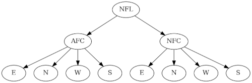
Each division has four teams. Adding each team under its division would make an awkwardly wide graph. I made a graph of the entire tree, rotated so that image is long rather than wide. Here’s a little piece of it.
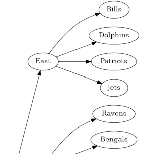
The full image is available here.
Geography
Now you may wonder how well the geographic division names correspond to geography. For example, the Dallas Cowboys are in the NFC East, and it’s a little jarring to hear Texas called “east.”
But within each conference, all the “East” teams are indeed east of all the West teams. And with one exception, all the North teams are indeed north of the South teams. The Indianapolis Colts are the exception. The Colts are in the AFC South, but are located to the north of the Cincinnati Bengals and the Baltimore Ravens in the AFC North.
This geographical sorting only applies within a conference. The Dallas Cowboys, for example are east of all the West teams within their conference, but they are west of the Kansas City Chiefs in the AFC West.
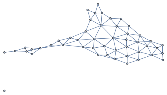
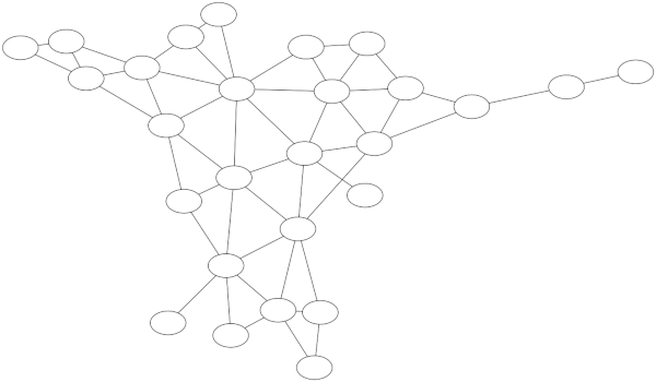
Here’s where topology comes in: you can make the division names match their geography if you morph the map of the United States pulling Indianapolis south of its geometric location.
Binary numbers
The graph structure of the NFL is essentially a full binary tree; you could make it into a binary tree by introducing a sub-conference layer and grouping the teams into pairs.
You could number the NFL teams with five bits: one for the conference, two for the division, and two more for the team. We could make the leading bit 0 for the AFC and 1 for the NFC. Then within each division, we could use 00 for East, 01 for North, 10 for West, and 11 for South. As mentioned above, this follows the mathematical convention of angles increasing counterclockwise starting at the positive x-axis.

The table above is an SVG image; here is the same data in plain text.


