Determining fundamental frequency

My daughter had a homework problem the other day that gave the frequencies of several Fourier components and asked her to find the fundamental frequency. The numbers were nice enough that brute force worked, and I’m sure that’s what students were expected to do. But this could easily be a much more sophisticated problem.

If the frequencies are all integers and exact multiples of a fundamental frequency, you can simply take the greatest common divisor of the frequencies. If you’re told the frequencies are 1760, 2200, and 3080, then the fundamental frequency is apparently 440 since that’s the greatest common divisor.

But what if the data are a little different? Say the highest pitch is 3081. Surely 440 should still be considered the fundamental frequency, even though now the greatest common divisor of the frequencies would be 1 Hz. What if the highest frequency was 3078 + π? Surely the fundamental frequency is still 440 for practical purposes.

And what might these practical purposes be? One purpose might be pitch detection. When several frequencies are combined that are small integer multiples of a fundamental frequency, we perceive the combination as having pitch given by that fundamental.

For something like a guitar string, the frequency components are close to small integer multiples of a fundamental frequency. But for something like a church bell, the frequencies don’t line up so neatly, though there’s still a clearly perceived pitch. For something like a metal mixing bowl, it may be difficulty to predict what pitch a person will hear when something strikes the bowl.

One complication we haven’t addressed yet is that the fundamental frequency will not be unique without some constraint. In the example above, the frequencies were all multiples of 440, but they’re also all multiples of 440/n for every positive integer n. We might get around this by specifying some lower bound on the fundamental frequency. Or we could say that all other things being equal, we want the largest candidate for the fundamental frequency.

We could formulate the problem of finding the fundamental frequency as an optimization problem. For example, we could form a mixed integer program. Suppose we have three frequencies f1, f2, and f3. We could find a fundamental frequency f and integers n1, n2, and n3 that minimize

(f1n1 f)² + (f2n2 f)² + (f3n3 f

subject to a lower bound on f.

We can eliminate the explicit dependence on the integer coefficients by minimizing

(f1/f − [f1/f])² + (f2/f − [f2/f])² + (f3/f − [f3/f])² .

where [x] denotes nearest integer to x. The first formulation has a more common form. The latter has a more complicated objective function, but it’s only a function of one variable.

Here’s what the latter looks like for frequencies 1760, 2200, and 3080.

objective function

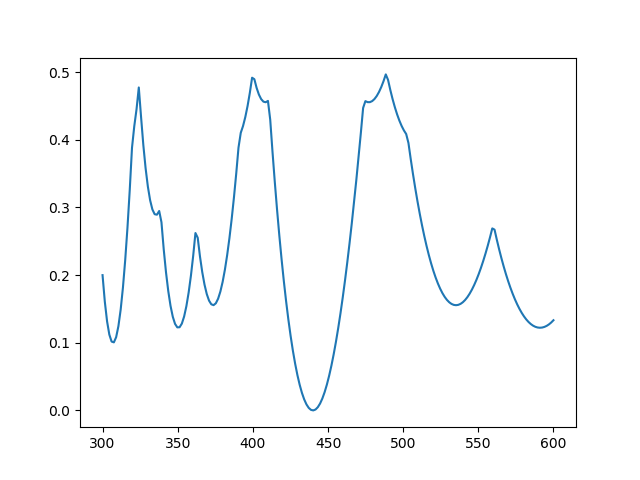
Clearly there’s a minimum at 440 Hz.

Here’s the same plot with 10% random noise [1] added to each frequency: 1701, 2368, and 3339.

objective function

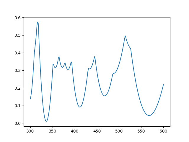
Now there’s a minimum near 336, but the local minimum at 566 is nearly as good.

Related posts

[1] There are a couple reasons you might want to solve a problem like this. Maybe your frequencies really are integer multiples of a fundamental frequency, but there is measurement error. Another is that the frequencies are not exactly multiples of a fundamental, as when striking a bell or a mixing bowl. How might you formulate the two cases differently?

Optimization, Dominoes, and Frankenstein

Robert Bosch has a new book coming out next week titled OPT ART: From Mathematical Optimization to Visual Design. This post will look at just one example from the book: creating images of Frankenstein’s monster [1] using dominoes.

Frankenstein made from 3 sets of double nine dominoes

The book includes two images, a low-resolution image made from 3 sets of dominoes and a high resolution image made from 48 sets. These are double nine dominoes rather than the more common double six dominoes because the former allow a more symmetric arrangement of dots. There are 55 dominoes in a double nine set. (Explanation and generalization here.)

Image of Frankenstein's monster made from 48 sets of double nine dominoes

The images are created by solving a constrained optimization problem. You basically want to use dominoes whose brightness is proportional to the brightness of the corresponding section of a photograph. But you can only use the dominoes you have, and you have to use them all.

You would naturally want to use double nines for the brightest areas since they have the most white spots and double blanks for the darkest areas. But you only have three of each in the first image, forty eight of each in the second, and you have to make do with the rest of the available pieces. So you solve an optimization problem to do the best you can.

Each domino can be places horizontally or vertically, as long as they fit the overall shape of the image. In the first image, you can see the orientation of the pieces if you look closely. Here’s a little piece from the top let corner.

Domino orientation

One double six is placed vertically in the top left. Next to it are another double six and a double five placed horizontally, etc.

There are additional constraints on the optimization problem related to contrast. You don’t just want to match the brightness of the photograph as well as you can, you also want to maintain contrast. For example, maybe a five-two domino would match the brightness of a couple adjacent squares in the photograph, but a seven-one would do a better job of making a distinction between contrasting regions of the image.

Bosch explains that the problem statement for the image using three sets of dominoes required 34,265 variables and 385 domino constraints. It was solved using 29,242 iterations of a simplex algorithm and required a little less than 2 seconds.

The optimization problem for the image created from 48 sets of dominoes required 572,660 variables and 5,335 constraints. The solution required 30,861 iterations of a simplex algorithm and just under one minute of computation.

Related posts

[1] In the Shelley’s novel Frankenstein, the doctor who creates the monster is Victor Frankenstein. The creature is commonly called Frankenstein, but strictly speaking that’s not his name. There’s a quote—I haven’t been able to track down its source—that says “Knowledge is knowing that Frankenstein wasn’t the monster. Wisdom is knowing that Frankenstein was the monster.” That is, the monster’s name wasn’t Frankenstein, but what Victor Frankenstein did was monstrous.

Something that bothers me about deep neural nets

Overfitting happens when a model does too good a job of matching a particular data set and so does a poor job on new data. The way traditional statistical models address the danger of overfitting is to limit the number of parameters. For example, you might fit a straight line (two parameters) to 100 data points, rather than using a 99-degree polynomial that could match the input data exactly and probably do a terrible job on new data. You find the best fit you can to a model that doesn’t have enough flexibility to match the data too closely.

Deep neural networks have enough parameters to overfit the data, but there are various strategies to keep this from happening. A common way to avoid overfitting is to deliberately do a mediocre job of fitting the model.

When it works well, the shortcomings of the optimization procedure yield a solution that differs from the optimal solution in a beneficial way. But the solution could fail to be useful in several ways. It might be too far from optimal, or deviate from the optimal solution in an unhelpful way, or the optimization method might accidentally do too good a job.

It a nutshell, the disturbing thing is that you have a negative criteria for what constitutes a good solution: one that’s not too close to optimal. But there are a lot of ways to not be too close to optimal. In practice, you experiment until you find an optimally suboptimal solution, i.e. the intentionally suboptimal fit that performs the best in validation.


One of my favorite proofs: Lagrange multipliers

One of my lightbulb moments in college was when my professor, Jim Vick, explained the Lagrange multiplier theorem. The way I’d seen it stated in a calculus text gave me no feel for why it should be true, but his explanation made sense immediately.

Suppose f(x) is a function of several variables, i.e. x is a vector, and g(x) = c is a constraint. Then the Lagrange multiplier theorem says that at the maximum of f subject to the constraint g we have ∇f = λ ∇g.

Where does this mysterious λ come from? And why should the gradient of your objective function be related to the gradient of a constraint? These seem like two different things that shouldn’t even be comparable.

Here’s the geometric explanation. The set of points satisfying g(x) = c is a surface. And for any k, the set of points satisfying f(x) = k is also surface. Imagine k very large, larger than the maximum of f on the surface defined by g(x) = c. You could think of the surface g(x) = c being a balloon inside the larger balloon  f(x) = k.

Now gradually decrease k, like letting the air out of the outer balloon, until the surfaces g(x) = c and f(x) = k first touch. At that point, the two surfaces will be tangent, and so their normal vectors, given by their gradients, point in the same direction. That is, ∇f and ∇g are parallel, and so ∇f is some multiple of ∇g. Call that multiple λ.

I don’t know how well that explanation works when written down. But when I heard Jim Vick explain it, moving his hands in the air, it was an eye-opener.

This is not a rigorous proof, and it does not give the most general result possible, but it explains what’s going on. It’s something to keep in mind when reading proofs that are more rigorous or more general. As I comment on here,

Proofs serve two main purposes: to establish that a proposition is true, and to show why it is true.

The literally hand-wavy proof scores low on the former criterion and high on the latter.

***

Jim Vick was a great teacher. Some of us affectionately called him The Grinning Demon because he was always smiling, even while he gave devilishly hard homework. He was Dean of Natural Sciences when I took a couple classes from him. He later became Vice President for Student Affairs and kept teaching periodically. He has since retired but still teaches.

After taking his topology course, several of us asked him to teach a differential geometry course. He hesitated because it’s a challenge to put together an undergraduate differential geometry course. The usual development of differential geometry uses so much machinery that it’s typically a graduate-level course.

Vick found a book that starts by looking only at manifolds given by level sets of smooth functions, like the surfaces discussed above. Because these surfaces sit inside a Euclidean space, you can quickly get to some interesting geometric results using elementary methods. We eventually got to the more advanced methods, but by then we had experience in a more tangible setting. As Michael Atiyah said, abstraction should follow experience, not precede it.

Natural optima occur in the middle

Akin’s eighth law of spacecraft design says

In nature, the optimum is almost always in the middle somewhere. Distrust assertions that the optimum is at an extreme point.

When I first read this I immediately thought of several examples where theory said that an optima was at an extreme, but experience said otherwise.

Linear programming (LP) says the opposite of Akin’s law. The optimal point for a linear objective function subject to linear constraints is always at an extreme point. The constraints form a many-sided shape—you could think of it something like a diamond—and the optimal point will always be at one of the corners.

Nature is not linear, though it is often approximately linear over some useful range. One way to read Akin’s law is to say that even when something is approximately linear in the middle, there’s enough non-linearity at the extremes to pull the optimal points back from the edges. Or said another way, when you have an optimal value at an extreme point, there may be some unrealistic aspect of your model that pushed the optimal point out to the boundary.

Related postData calls the model’s bluff

Example of not inverting a matrix: optimization

People are invariably surprised when they hear it’s hardly ever necessary to invert a matrix. It’s very often necessary solve linear systems of the form Ax = b, but in practice you almost never do this by inverting A. This post will give an example of avoiding matrix inversion. I will explain how the Newton-Conjugate Gradient method works, implemented in SciPy by the function fmin_ncg.

If a matrix A is large and sparse, it may be possible to solve Ax = b but impossible to even store the matrix A−1 because there isn’t enough memory to hold it. Sometimes it’s sufficient to be able to form matrix-vector products Ax. Notice that this doesn’t mean you have to store the matrix A; you have to produce the product Ax as if you had stored the matrix A and multiplied it by x.

Very often there are physical reasons why the matrix A is sparse, i.e. most of its entries are zero and there is an exploitable pattern to the non-zero entries. There may be plenty of memory to store the non-zero elements of A, even though there would not be enough memory to store the entire matrix. Also, it may be possible to compute Ax much faster than it would be if you were to march along the full matrix, multiplying and adding a lot of zeros.

Iterative methods of solving Ax = b, such as the conjugate gradient method, create a sequence of approximations that converge (in theory) to the exact solution. These methods require forming products Ax and updating x as a result. These methods might be very useful for a couple reasons.

  1. You only have to form products of a sparse matrix and a vector.
  2. If don’t need a very accurate solution, you may be able to stop very early.

In Newton’s optimization method, you have to solve a linear system in order to find a search direction. In practice this system is often large and sparse. The ultimate goal of Newton’s method is to minimize a function, not to find perfect search directions. So you can save time by finding only approximately solutions to the problem of finding search directions. Maybe an exact solution would in theory take 100,000 iterations, but you can stop after only 10 iterations! This is the idea behind the Newton-Conjugate Gradient optimization method.

The function scipy.optimize.fmin_ncg can take as an argument a function fhess that computes the Hessian matrix H of the objective function. But more importantly, it lets you provide instead a function fhess_p that computes the product of the H with a vector. You don’t have to supply the actual Hessian matrix because the fmin_ncg method doesn’t need it. It only needs a way to compute matrix-vector products Hx to find approximate Newton search directions.

For more information, see the SciPy documentation for fmin_ncg.

More: Applied linear algebra

Moore’s law squared

In a review of linear programming solvers from 1987 to 2002, Bob Bixby says that solvers benefited as much from algorithm improvements as from Moore’s law.

Three orders of magnitude in machine speed and three orders of magnitude in algorithmic speed add up to six orders of magnitude in solving power. A model that might have taken a year to solve 10 years ago can now solve in less than 30 seconds.

Source: In Pursuit of the Traveling Salesman

Related post: A brief note on Moore’s law

Designed from the inside out

The most recent episode of the Plus Maths podcast describes how the London Velodrome was designed. Being a math podcast, it focuses on the optimization problems involved in the design and the finite element modeling of the structure.

The beautiful shape of the building was not an initial goal but rather a consequence of design decisions that began with the track and worked outward.

It’s perhaps surprising, given the pragmatic design concerns of optimizing the experience of people using the velodrome, maximizing the efficiency of the building, all within the constraints of the construction methods, the design process has led to a stunningly beautiful roof that almost echos the shape of the track.

… it’s a happy by-product of the design. There was nothing intentional in the design [of the roof] that we wanted it to look like the track. … it’s the opposite if the track …

Image by Richard Davies via the Plus Math article How the velodrome found its form.

Related post: Mathematics behind the Olympic water cube

Markov chains don’t converge

I often hear people often say they’re using a burn-in period in MCMC to run a Markov chain until it converges. But Markov chains don’t converge, at least not the Markov chains that are useful in MCMC. These Markov chains wander around forever exploring the domain they’re sampling from. Any point that makes a “bad” starting point for MCMC is a point you might reach by burn-in.

Not only that, Markov chains can’t remember how they got where they are. That’s their defining property. So if your burn-in period ends at a point x, the chain will perform exactly as if you had simply started at x.

When someone says a Markov chain has converged, they may mean that the chain has entered a high-probability region. I’ll explain in a moment why that’s desirable. But the belief/hope is that a burn-in period will put a Markov chain in a high-probability region. And it probably will, but there are a couple reasons why this isn’t necessarily the best thing to do.

  1. Burn-in may be inefficient. Casting aside worries that burn-in may not do what you want, it can be an inefficient way to find a high-probability region. MCMC isn’t designed to optimize a density function but rather to sample from it.

Why use burn-in? MCMC practitioners often don’t know how to do optimization, and in any case the corresponding optimization problem may be difficult. Also, if you’ve got the MCMC code in hand, it’s convenient to use it to find a starting point as well as for sampling.

So why does it matter whether you start your Markov chain in a high-probability region? In the limit, it doesn’t matter. But since you’re averaging some function of some finite number of samples, your average will be a better approximation if you start at a typical point in the density you’re sampling. If you start at a low probability location, your average may be more biased.

Samples from Markov chains don’t converge, but averages of functions applied to these samples may converge. When someone says a Markov chain has converged, they may mean they’re at a point where the average of a finite number of function applications will be a better approximation of the thing they want to compute than if they’d started at a low probability point.

It’s not just a matter of imprecise language when people say a Markov chain has converged. It sometimes betrays a misunderstanding of how Markov chains work.