A recipe for creating random fractals

Last week I gave an example of a randomly generated fractal and mentioned that it was “a particularly special case of a more general algorithm for generating similar fractals found in [1].”

Here’s the general pattern. First, create a non-singular matrix M with integer entries and let k be the determinant of M.

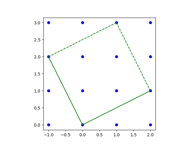
Let P be the parallelogram spanned by the columns of M. Choose a set of column vectors ri for i = 1, 2, 3, …, k from the two columns of M and from the interior of P.

Pick a random starting vector v then iterate

vM−1 vri

where i is chosen at random on each iterations.

Here’s an example suggested as an exercise in [2]. We start with

M = \begin{bmatrix} 2 & -1 \\ 1 & \phantom{-}2 \end{bmatrix}

and look at the parallelogram spanned by the columns of M.

NB: The initial version of this post had an error in the grid, which led to an error in the code, and produced a different fractal.

Then the algorithm described above is implemented in the following Python code.

import numpy as np
import matplotlib.pyplot as plt

A = np.linalg.inv(np.array([[2,  -1], [1, 2]]))
R = np.array([[2, -1, 0,  1, 1],
              [1,  2, 2,  2, 1]])

v = np.random.random(size=2)
for _ in range(100000):
    i = np.random.choice([0, 1, 2, 3, 4])
    v = np.dot(A, v) + R[:, i]
    plt.plot(v[0], v[1], 'bo', markersize=1)
plt.gca().set_aspect("equal")
plt.show()

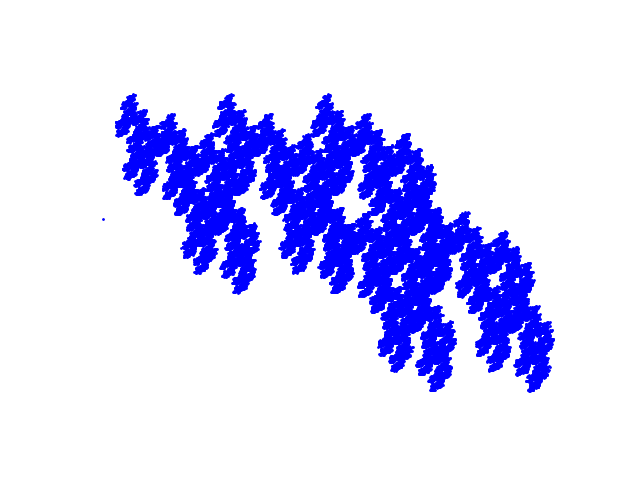
This produces the following fractal.

[1] Darst, Palagallo, and Price. Fractal Tilings in the Plane. Mathematics Magazine [71]:1, 1998.

[2] Lorelei Koss, Fractal Rep-tiles and Geometric Series. Math Horizons. Vol 30, Issue 1, September 2022.

Base58Check encoding in Python

The previous post began by saying “Bitcoin’s Wallet Import Format (WIF) is essentially Base58 encoding with a checksum.” More specifically, WIF uses Base58Check encoding.

This post will fill in the missing details and show how to carry out computing Base58Check in Python. There are multiple ways to stub your toe doing this because it involves encoding issues. You have to compute hash functions, which are conceptually easy, but you get into issues of converting strings into bytes, byte order, endianness, etc. And in Python, the output of a hash isn’t a number or a string, but a object that you have to “digest” one way or another. Then there’s getting the syntax just right to do the Base58 encoding.

This post will step through this tutorial example.

***

The example says to take the SHA256 hash of

    800C28FCA386C7A227600B2FE50B7CAE11EC86D3BF1FBE471BE89827E19D72AA1D

and get

    8147786C4D15106333BF278D71DADAF1079EF2D2440A4DDE37D747DED5403592

OK, here we go:

>>> from hashlib import sha256
>>> s = "800C28FCA386C7A227600B2FE50B7CAE11EC86D3BF1FBE471BE89827E19D72AA1D"
>>> d = bytes.fromhex(s)
>>> sha256(d).hexdigest().upper()
'8147786C4D15106333BF278D71DADAF1079EF2D2440A4DDE37D747DED5403592'

This matches what we were supposed to get.

Next the sample says to hash the result again. We have to hash the bytes of the first hash, not the string representation.

>>> sha256(sha256(d).digest()).hexdigest().upper()
'507A5B8DFED0FC6FE8801743720CEDEC06AA5C6FCA72B07C49964492FB98A714'

The output matches what the example says we should get.

Now we’re supposed to take the first 4 bytes (represented by the first 8 hex characters) and stick them on the end of the address we stored as s above.

s += '507A5B8D'

And finally we’re supposed to convert the result to Base58.

>>> from base58 import b58encode
>>> b58encode(bytes.fromhex(s))
b'5HueCGU8rMjxEXxiPuD5BDku4MkFqeZyd4dZ1jvhTVqvbTLvyTJ'

This matches the result in the example.

Perpetual Calendars

The previous post explained why the Gregorian calendar is the way it is, and that it consists of a whole number of weeks. It follows that the Gregorian calendar repeats itself every 400 years. For example, the calendar for 2025 will be exactly the same as the calendar for 1625 and 2425.

There are only 14 possible printed calendars, if you don’t print the year on the calendar. There are seven possibilities for the day of the week for New Year’s Day, and there are two possibilities for whether the year is a leap year.

A perpetual calendar is a set of the 14 possible calendars, along with some index that tells which possible calendar is appropriate in a given year.

Are each of the 14 calendars equally frequent? Almost, aside from the fact that leap years are less frequent. Each ordinary year calendar occurs 43 or 44 times, and each leap year calendar occurs 13, 14, or 15 times.

Related posts

MD5 hash collision example

Marc Stevens gave an example of two alphanumeric strings that differ in only one byte that have the same MD5 hash value. It may seem like beating a dead horse to demonstrate weaknesses in MD5, but it’s instructive to study the flaws of broken methods. And despite the fact that MD5 has been broken for years, lawyers still use it.

The example claims that

TEXTCOLLBYfGiJUETHQ4hAcKSMd5zYpgqf1YRDhkmxHkhPWptrkoyz28wnI9V0aHeAuaKnak

and

TEXTCOLLBYfGiJUETHQ4hEcKSMd5zYpgqf1YRDhkmxHkhPWptrkoyz28wnI9V0aHeAuaKnak

have the same hash value.

This raises several questions.

Are these two strings really different, and if so, how do they differ? If you stare at the strings long enough you can see that they do indeed differ by one character. But how could you compare long strings like this in a more automated way?

How could you compute the MD5 hash values of the strings to verify that they are the same?

The following Python code addresses the questions above.

from hashlib import md5
from difflib import ndiff

def showdiff(a, b):
    for i,s in enumerate(ndiff(a, b)):
        if s[0]==' ': continue
        elif s[0]=='-':
            print(u'Delete "{}" from position {}'.format(s[-1],i))
        elif s[0]=='+':
            print(u'Add "{}" to position {}'.format(s[-1],i))    

a = "TEXTCOLLBYfGiJUETHQ4hAcKSMd5zYpgqf1YRDhkmxHkhPWptrkoyz28wnI9V0aHeAuaKnak"
b = "TEXTCOLLBYfGiJUETHQ4hEcKSMd5zYpgqf1YRDhkmxHkhPWptrkoyz28wnI9V0aHeAuaKnak"

showdiff(a, b)

ahash = md5(a.encode('utf-8')).hexdigest()
bhash = md5(b.encode('utf-8')).hexdigest()
assert(ahash == bhash)

The basis of the showdiff function was from an answer to a question on Stack Overflow.

The output of the call to showdiff is as follows.

Delete "A" from position 21
Add "E" to position 22

This means we can form string b from a by changing the ‘A’ in position 21 to an ‘E’. There was only one difference between the two strings in this example, but showdiff could be useful for understanding more complex differences.

The assert statement passes because both strings hash to faad49866e9498fc1719f5289e7a0269.

Related posts

Finite differences and Pascal’s triangle

The key to solving a lot of elementary what-number-comes-next puzzles is to take first or second differences. For example, if asked what the next item in the series

14, 29, 50, 77, 110, …

the answer (or at lest the answer the person posing the question is most likely looking for) is 149. You might discover this by first looking at the differences of the items:

15, 21, 27, 33, …

The differences all differ by 6, i.e. the second difference of the series is constant. From there you can infer that the next item in the original series will be 39 more than the previous, i.e. it will be 149.

We can apply the same technique for exploring series that are not artificial puzzles. For example, a one-page article by Harlan Brothers [1] asks what would happen if you looked at the products of elements in each row of Pascal’s triangle.

The products grow very quickly, which suggests we work on a log scale. Define

s(n) = \log \prod{k=0}^n \binom{n}{k}  = \sum_{k=0}^n \log \binom{n}{k}

Let’s use a little Python script to look at the first 10 elements in the series.

    from scipy.special import binom
    from numpy import vectorize, log

    def s(n):
        return sum([log(binom(n, k)) for k in range(n+1)])
    s = vectorize(s)

    n = range(1, 11)
    x = s(n)
    print(x)

This prints

0.
0.69314718
2.19722458
4.56434819
7.82404601
11.9953516
17.0915613
23.1224907
30.0956844
38.0171228

Following the strategy at the top of the post, let’s look at the first differences of the sequence with [2]

    y = x[1:] - x[:-1]
    print(y)

This prints

0.69314718
1.50407740
2.36712361
3.25969782
4.17130560
5.09620968
6.03092943
6.97319372
7.92143836

The first differences are increasing by about 0.9, i.e. the second differences are roughly constant. And if we look at the third differences, we find that they’re small and getting smaller the further out you go.

We can easily look further out in the sequence by changing range(1, 11) to range(1, 101). When we do, we find that the second difference are

…, 0.99488052, 0.9949324. 0.99498325

If we look even further out, looking at a thousand terms, the last of the second differences is

…, 0.99949883, 0.99949933, 0.99949983

We might speculate that the second differences are approaching 1 as n → ∞. And this is exactly what is proved in [1], though the author does not work on the log scale. The paper shows that the ratio of the ratio of consecutive lines converges to e. This is equivalent on a log scale to saying the second differences converge to 1.

[1] Harlan J. Brothers. Math Bite: Finding e in Pascal’s Triangle. Mathematics Magazine , Vol. 85, No. 1 (February 2012), p. 51

[2] In Python, array elements are numbered starting at 0, and x[1:] represents all but the first elements of x. The index −1 is a shorthand for the last element, so x{:-1] means all the elements of x up to (but not including) the last.

Factoring pseudoprimes

Fermat’s little theorem says that if p is a prime number, then for any positive integer b < p we have

bp−1 = 1 (mod p).

This theorem gives a necessary but not sufficient condition for a number to be prime.

Fermat’s primality test

The converse of Fermat’s little theorem is not always true, but it’s often true. That is, if there exists some base 1 < b < n such that

bn−1 = 1 (mod n)

then n is likely to be prime. There are examples where the equation above holds for a pair (b, n) even though n is not prime, and in that case n is called a pseudoprime to the base b.

If you’re searching for large primes, say for use in encryption, then you’d begin by applying Fermat’s little theorem with a few small values of b. This is because although Fermat’s test can’t prove that a number is prime, it can prove that a number is not prime.

For a small example, suppose you wanted to test whether 50621 is prime. You could start by applying Fermat’s test with b = 2 as in the following Python code.

>>> n = 50621
>>> 2**(n−1) % n
9605

Since the result is not 1, we know 50621 is not prime. This doesn’t tell us what the factors of 50621 are, but we know that it has nontrivial factors. We say 2 is a witness that the number 50621 is not prime.

Next, let’s see whether 294409 might be prime.

>>> n = 294409
>>> 2**(n – 1) % n
1

This tells us 294409 might be prime. It has passed a test that filters out a lot of composite numbers. What now? We could try other values of b: 3, 5, 7, 11, …. This will not resolve the question of whether 294409 is prime unless we keep going until we try 37. And in fact 37 is the smallest factor of 294409. Our number 294409 is a Carmichael number, a composite number n that passes Fermat’s primality test for all bases b relatively prime to n.

Note that it would be more efficient to use pow(b, n − 1, n) rather than 2**(n − 1) % n because the former takes advantage of the fact that we don’t need to compute 2n−1 per se and can reduce all intermediate calculations mod n.

Factoring pseudoprimes

Now suppose we have a number n that has passed Fermat’s primality test for some base b and we suspect that n is a pseudoprime. If we want to (try to) factor n, knowing that it is a pseudoprime to the base b gives us a head start. We can exploit the fact that we know b to factor n in polynomial time, unless n is a strong pseudoprime.

Suppose we have a number n that we suspect is a pseudoprime to the base b, and we’re smart enough to at least check that n is an odd number, then we begin by pulling out all the factors of 2 that we can from n − 1:

n − 1 = 2e f.

Next consider the set of numbers

bkf

for k = 1, 2, 4, …, 2e. Let x be the smallest of these numbers which is not congruent to 1 mod n. The existence of such an x is essentially the definition of strong pseudoprime [1].

Then gcd(x − 1, n) and gcd(x + 1, n) are factors of n. This is theorem 10.4 of [2].

Python example

Let n = 873181. This is a pseudoprime to the base b = 3, which we can confirm by seeing that pow(3, n−1, n) returns 1.

Now 873180 is divisible by 4 but not by 8, so e = 2. So the theorem above says we should compute

>>> b, e = 3, 2
>>> [pow(b, f*2**k, n) for k in range(e+1)]

This produces [2643, 1, 1]. So x = 2643,

>> x = 2643
>>> from sympy import gcd
>>> gcd(x−1, n)
1321
>>> gcd(x+1, n)
661

shows that 1321 and 661 are both factors of 873181.

Related posts

[1] Definition of strong pseudoprime. A strong pseudo prime to base b is a composite odd integer m such that if m − 1 = 2ef  with f odd, then either bf = 1 (mod m) or bf2c ≡ −1 (mod m) for some 0 ≤ c < e.

[2] The Joy of Factoring by Samuel S. Wagstaff, Jr.

Computing inverse factorial

I needed the inverse factorial function for my previous post. I was sure I’d written a post on computing the inverse factorial, and intended to reuse the code from that earlier post. But when I searched I couldn’t find anything, so I’m posting the code here for my future reference and for anyone else who may need it.

Given a positive number x, how can you find a number n such that n! = x, or such that n! ≈ x?

Mathematical software tends to work with the gamma function rather than factorials because Γ(x) extends x! to real numbers, with the relation Γ(x+1) = x!. The left side is often taken as a definition of the right side when x is not a positive integer.

Not only do we prefer to work with the gamma function, it’s easier to work with the logarithm of the gamma function to avoid overflow.

The Python code below finds the inverse of the log of the gamma function using the bisection method. This method requires an upper and lower bound. If we only pass in positive values, 0 serves as a lower bound. We can find an upper bound by trying powers of 2 until we get something large enough.

from scipy.special import gammaln
from scipy.optimize import bisect

def inverse_log_gamma(logarg):
    assert(logarg > 0)
    a = 1
    b = 2
    while b < logarg:
        b = b*2
    return bisect(lambda x: gammaln(x) - logarg, a, b)

def inverse_factorial(logarg):
    g = inverse_log_gamma(logarg)
    return round(g)-1 

Note that the inverse_factorial function takes the logarithm of the value whose inverse factorial you want to compute.

For example,

inverse_factorial(log(factorial(42))))

returns 42.

Working on the log scale lets us work with much larger numbers. The factorial of 171 is larger than the largest IEEE double precision number, and so inverse_factorial could not return any value larger than 171 if we passed in x rather than log x. But by taking log x as the argument, we can calculate inverse factorials of numbers so large that the factorial overflows.

For example, suppose we want to find the value of m such that m! is the closest factorial to √(2024!), as we did in the previous post. We can use the code

inverse_factorial(gammaln(2025)/2)

to find m = 1112 even though 1112! is on the order of 102906, far larger than the largest representable floating point number, which is on the order of 10308.

When n! = x does not have an exact solution, there is some choice over what value of n to return as the inverse factorial of x. The code above minimizes the distance from n! to x on a log scale. You might want to modify the code to minimize the distance on a linear scale, or to find the largest n with n! < x, or the smallest n with n! > x depending on your application.

Related posts

Kepler triangle

A Kepler triangle is a right triangle whose sides are in geometric progression. That is, if the sides have length a < b < c, then b/a = c/b = k.

All Kepler triangles are similar because the proportionality constant k can only take on one value. To see this, we first pick our units so that a = 1. Then b = k and c = k². By the Pythagorean theorem

a² + b² = c²

and so

1 + k2 = k4

which means k² equals the golden ratio φ.

Here’s a nice geometric property of the Kepler triangle proved in [1].

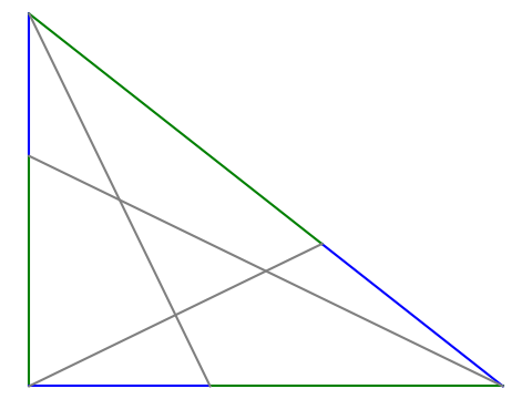
Go around the triangle counterclockwise placing a point on each side dividing the side into pieces that are in golden proportion. Connect these three points with the opposite vertex. Then the triangle formed by the intersections of these line segments is also a Kepler triangle.

On each side, the ratio of the length of the green segment to the blue segment is φ. The grey triangle in the middle is another Kepler triangle.

The rest of this post will present the code that was used to create the image above.

We’ll need the following imports.

import matplotlib.pyplot as plt
from numpy import array
from numpy.linalg import solve

We’ll also need to define the golden ratio, a function to split a line segment into golden proportions, and a function to draw a line between two points.

φ = (1 + 5**0.5)/2

def golden_split(pt1, pt2):
    return (1/φ)*pt1 + (1 - 1/φ)*pt2

def connect(pt1, pt2, style):
    plt.plot([pt1[0], pt2[0]], [pt1[1], pt2[1]], style)

Now we can draw the figure.

A = array([0, 1])
B = array([0, 0])
C = array([φ**0.5, 0])

X = golden_split(A, B)
Y = golden_split(B, C)
Z = golden_split(C, A)

connect(A, X, "b")
connect(X, B, "g")
connect(B, Y, "b")
connect(Y, C, "g")
connect(C, Z, "b")
connect(Z, A, "g")
connect(A, Y, "grey")
connect(B, Z, "grey")
connect(C, X, "grey")

plt.gca().set_aspect("equal")
plt.axis("off")
plt.show()

We can show algebraically that the golden_split works as claimed, but here is a numerical illustration.

assert(abs( (C[0] - Y[0]) / (Y[0] - A[0]) - φ) < 1e-14)

Similarly, we can show numerically what [1] proves exactly, i.e. that the triangle in the middle is a Kepler triangle.

from numpy.linalg import solve, norm

def intersect(pt1, pt2, pt3, pt4):
    # Find the intersection of the line joining pt1 and pt2
    # with the line joining pt3 and pt4.
    m1 = (pt2[1] - pt1[1])/(pt2[0] - pt1[0])
    m3 = (pt4[1] - pt3[1])/(pt4[0] - pt3[0])
    A = array([[m1, -1], [m3, -1]])
    rhs = array([m1*pt1[0]-pt1[1], m3*pt3[0]-pt3[1]])
    x = solve(A, rhs)
    return x

I = intersect(A, Y, C, X)
J = intersect(A, Y, B, Z)
K = intersect(B, Z, C, X)

assert( abs( norm(I - J)/norm(J - K) - φ**0.5 ) < 1e-14 )
assert( abs( norm(I - K)/norm(I - J) - φ**0.5 ) < 1e-14 )

Related posts

[1] Jun Li. Some properties of the Kepler triangle. The Mathematical Gazette, November 2017, Vol. 101, No. 552, pp. 494–495

Cross-platform way to enter Unicode characters

The previous post describes the hoops I jumped through to enter Unicode characters on a Mac. Here’s a script to run from the command line that will copy Unicode characters to the system clipboard. It runs anywhere the Python module pyperclip runs.

    #!/usr/bin/env python3

    import sys
    import pyperclip

    cp = sys.argv[1]
    ch = eval(f"chr(0x{cp})")
    print(ch)
    pyperclip.copy(ch)

I called this script U so I could type

    U 03c0

at the command line, for example, it would print π to the command line and also copy it to the clipboard.

Unlike the MacOS solution in the previous post, this works for any Unicode value, i.e. for code points above FFFF.

On my Linux box I had to install xclip before pyperclip would work.

Curvature at Cairo

I was flipping through Gravitation [1] this weekend and was curious about an illustration on page 309. This post reproduces that graph.

The graph is centered at Cairo, Egypt and includes triangles whose side lengths are the distances between cities. The triangles are calculated using only distances, not by measuring angles per se.

The geometry of each triangle is Euclidean: giving the three edge lengths fixes all the features of the figure, including the indicated angle. … The triangles that belong to a given vertex [i.e. Cairo], laid out on a flat surface, fail to meet.

I will reproduce the plot in Python because I’m more familiar with making plots there. But I’ll get the geographic data out of Mathematica, because I know how to do that there.

Geographic information from Mathematica

I found the distances between the various cities using the GeoDistance function in Mathematica. The arguments to GeoDistance are “entities” which are a bit opaque. When using Mathematica interactively, you can use ctrl + = to enter the name of an entity. There’s some guesswork, e.g. whether I meant New York City or the state of New York when I entered “New York”, but Mathematica guessed correctly. The following code lists the city entities explicitly.

    cities = {
        Entity["City", {"Cairo", "Cairo", "Egypt"}], 
        Entity["City", {"Delhi", "Delhi", "India"}], 
        Entity["City", {"Moscow", "Moscow", "Russia"}], 
        Entity["City", {"Brussels", "Brussels", "Belgium"}], 
        Entity["City", {"Reykjavik", "Hofudhborgarsvaedhi", "Iceland"}], 
        Entity["City", {"NewYork", "NewYork", "UnitedStates"}], 
        Entity["City", {"CapeTown", "WesternCape", "SouthAfrica"}], 
        Entity["City", {"PortLouis", "PortLouis", "Mauritius"}] }

Most of these are predictable, but I would not have guessed the code for Reykjavik or Cape Town. I found these by using the command InputForm and entering the entities as above.

I found the distance from Cairo to each of the other cities with

    Table[GeoDistance[cities[[1]], cities[[i]]], {i, 2, 8}]

and the distances from the cities to their neighbors with

    Table[GeoDistance[cities[[i]], cities[[i + 1]]], {i, 2, 7}]
    GeoDistance[cities[[8]], cities[[2]]]

Drawing the plot

Now that we’ve got the data, how do we draw the plot?

Let’s put Cairo at the origin. First we draw a line from Cairo to Delhi. We might as well put Delhi on the x-axis to make things simple.

Next we need to plot Moscow. We know the distance R1 from Cairo to Moscow, and the distance R2 from Delhi to Moscow. So imagine drawing a circle of radius R1 centered at Cairo and a circle of radius R1 centered at Delhi. Moscow is located where the two circles intersect. The previous post shows how to find the intersection of circles.

The two circles intersect in at two points, so which do we choose? We choose the intersection point that preserves the orientation of the original graph (and the globe). As we go through the cities in counterclockwise order, the cross product of the previous line to the next line should have positive z component.

This shows that the original graph was not to scale, though the gap between triangles was approximately to scale. In hindsight this should have been obvious: Brussels and Reykjavik are much closer to each other than Capetown and New York are.

The gap

Why the gap? Because the earth is curved at Cairo (and everywhere else). If the earth were flat, the triangles would fit together without any gaps.

There’s no gap when you take spherical triangles on the globe. But even though the triangles preserve length when projected to the plane, they cannot preserve angles too. The sum of the angles in a spherical triangle adds up to more than 180°, and the amount by which the sum exceeds 180° is proportional to the size of the spherical triangle. Since the angles of triangles in the plane do add up to 180°, each flat triangle fails to capture a bit of the corresponding spherical triangles, and the failures add up to the gap we see in the image.

[1] Gravitation by Misner, Thorne, and Wheeler. 1973.