Golden integration

Let φ be the golden ratio. The fractional parts of nφ bounce around in the unit interval in a sort of random way. Technically, the sequence is quasi-random.

Quasi-random sequences are like random sequences but better in the sense that they explore a space more efficiently than random sequences. For this reason, Monte Carlo integration (“integration by darts“) can often be made more efficient by replacing random sequences with quasi-random sequence. This post will illustrate this efficiency advantage in one dimension using the fractional parts of nφ.

Here are functions that will generate our integration points.

    from numpy import random, zeros

    def golden_source(n):
        phi = (1 + 5**0.5)/2
        return (phi*n)%1

    def random_source(N):
        return random.random()

We will pass both of these generators as arguments to the following function which saves a running average of function evaluates at the generated points.

    def integrator(f, source, N):
        runs = zeros(N)
        runs[0] = f(source(0))
        for n in range(1, N):
            runs[n] = runs[n-1] + (f(source(n)) - runs[n-1])/n
        return runs

We’ll use as our example integrand f(x) = x² (1 – x)³. The integral of this function over the unit interval is 1/60.

    def f(x):
        return x**2 * (1-x)**3
    exact = 1/60

Now we call our integrator.

    random.seed(20230429)
    N = 1000
    golden_run = integrator(f, golden_source, N)
    random_run = integrator(f, random_source, N)

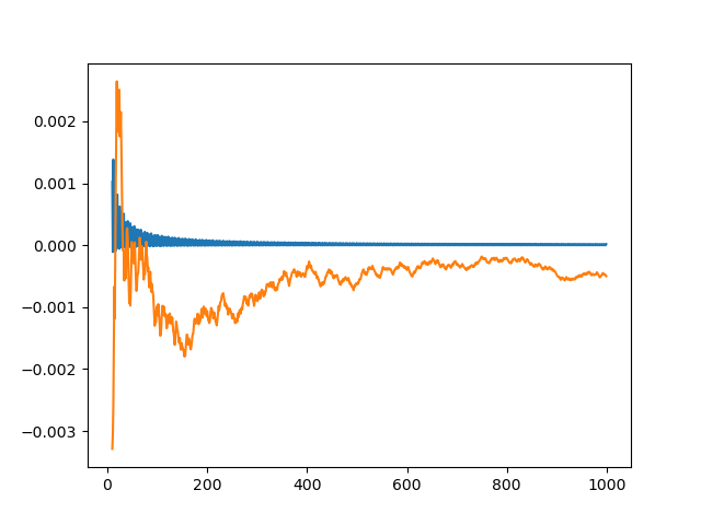
Now we plot the difference between each run and the exact value of the integral. Both methods start out with wild fluctuations. We leave out the first 10 elements in order to make the error easier to see.

    import matplotlib.pyplot as plt

    k = 10
    x = range(N)
    plt.plot(x[k:], golden_run[k:] - exact)
    plt.plot(x[k:], random_run[k:] - exact)

This produces the following plot.

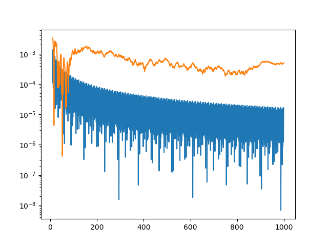
The integration error using φn – ⌊φn⌋ is so close to zero that it’s hard to observe its progress. So we plot it again, this time taking the absolute value of the integration error and plotting on a log scale.

    plt.plot(x[k:], abs(golden_run[k:] - exact))
    plt.plot(x[k:], abs(random_run[k:] - exact))
    plt.yscale("log")

This produces a more informative plot.

The integration error for the golden sequence is at least an order of magnitude smaller, and often a few orders of magnitude smaller.

The function we’ve integrated has a couple features that make integration using quasi-random sequences (QMC, quasi-Monte Carlo) more efficient. First, it’s smooth. If the integrand is jagged, QMC has no advantage over MC. Second, our integrand could be extended smoothly to a periodic function, i.e. f(0) = f(1) and f′(0) = f′(1). This makes QMC integration even more efficient.

Related posts

Elliptic functions of a complex argument in Python

I used Mathematica to create the graphics for my previous two posts because SciPy didn’t have the functions I needed. In particular, elliptic integrals and elliptic functions in SciPy only take real-valued arguments, but I needed to use complex arguments. Also, I needed theta functions, which are not in SciPy at all.

I thought mpmath might have the functions I wanted, and indeed it does.

Function names are slightly different between mpmath and SciPy. For example, the ellipe function in mpmath is overloaded to compute the complete elliptic integral of the first kind if given one argument and the incomplete counterpart if given two arguments.

The mpmath library works with arbitrary precision by default, and returns its own numeric types. But you can prefix a function with fp. in order to get a Python floating point value back. For example,

>>> import mpmath as mp
>>> mp.ellipe(1+1j, 1)
mpc(real='1.2984575814159773', imag='0.63496391478473613')
>>> mp.fp.ellipe(1+1j, 1)
(1.2984575814159773+0.634963914784736j)

When a cubic or quartic has a double root

Thanks to the quadratic equation, it’s easy to tell whether a quadratic equation has a double root. The equation

ax^2 + bx + c = 0

has a double root if and only if the discriminant

b^2 - 4ac

is zero.

The discriminant of a cubic is much less known, and the analogs for higher order polynomials are unheard of. There is a discriminant for polynomials of all degrees, though the complexity of the discriminant grows quickly with the degree of the polynomial.

This post will derive the discriminant of a cubic and a quartic.

Resultants

The resultant of a pair of polynomials is zero if and only if the two polynomials have a common root. Resultants have come up in a couple previous posts about solving trigonometric equations.

A polynomial p(x) has a double root if p and its derivative p‘ are both zero somewhere. The discriminant of p is the resultant of p and p’.

The resultant of two polynomials is a determinant of their Sylvester matrix. This matrix is easier to describe by example than by equation. You basically fill a matrix with shifts of the coefficients of both polynomials and fill in the gaps with zeros.

MathWorld gives the following Mathematica code for the Sylvester matrix of two inputs.

    SylvesterMatrix1[poly1_, poly2_,  var_] :=
      Function[{coeffs1, coeffs2}, With[
        {l1 = Length[coeffs1], l2 = Length[coeffs2]},
          Join[
            NestList[RotateRight, PadRight[coeffs1,
              l1 + l2 -  2], l2 - 2],
            NestList[RotateRight, PadRight[coeffs2,
              l1 + l2 - 2], l1 - 2]
          ]
        ]
      ][
        Reverse[CoefficientList[poly1, var]],
        Reverse[CoefficientList[poly2, var]]
    ]

Cubic discriminant

If we apply this to the cubic polynomial

ax^3 + bx^2 + dx + c

we get the following matrix.

\left( \begin{array}{ccccc} a & b & c & d & 0 \\ 0 & a & b & c & d \\ 3 a & 2 b & c & 0 & 0 \\ 0 & 3 a & 2 b & c & 0 \\ 0 & 0 & 3 a & 2 b & c \\ \end{array} \right)

We can compute the resultant by taking the determinant of the above matrix.

    g[x_] := a x^3 + b x^2 + c x + d
    SylvesterMatrix1[g[x], D[g[x], x], x]

We get the following result

-a b^2 c^2 + 4 a^2 c^3 + 4 a b^3 d - 18 a^2 b c d + 27 a^3 d^2

and we can verify that this is the same result we would get from calling the Resultant directly with

    Resultant[g[x], D[g[x], x], x]

Although the resultant is defined in terms of a determinant, that doesn’t mean that resultants are necessarily computed by computing determinants. The Sylvester matrix is a very special matrix, and there are clever ways to exploit its structure to create more efficient algorithms.

Each term in the resultant has a factor of a, and the discriminant is the resultant divided by –a.

Quartic discriminant

Now let’s repeat our exercise for the quartic. The Sylvester matrix for the quartic polynomial

ax^4 + bx^3 + cx^2 + dx + e

and its derivative is

\left( \begin{array}{ccccccc} a & b & c & d & e & 0 & 0 \\ 0 & a & b & c & d & e & 0 \\ 0 & 0 & a & b & c & d & e \\ 4 a & 3 b & 2 c & d & 0 & 0 & 0 \\ 0 & 4 a & 3 b & 2 c & d & 0 & 0 \\ 0 & 0 & 4 a & 3 b & 2 c & d & 0 \\ 0 & 0 & 0 & 4 a & 3 b & 2 c & d \\ \end{array} \right)

I created the image above with the following Mathematica code.

    f[x_] := a x^4 + b x^3 + c x^2 + d x + e
    TeXForm[SylvesterMatrix1[f[x], D[f[x], x], x]]

If we take the determinant, we get the resultant, but it’s a mess.

256 a^4 e^3-192 a^3 b d e^2-128 a^3 c^2 e^2+144 a^3 c d^2 e \\ -27 a^3 d^4+144 a^2 b^2 c e^2-6 a^2 b^2 d^2 e-80 a^2 b c^2 d e \\ +18 a^2 b c d^3+16 a^2 c^4 e-4 a^2 c^3 d^2-27 a b^4 e^2\\ +18 a b^3 c d e -4 a b^3 d^3 -4 a b^2 c^3 e+a b^2 c^2 d^2

Again each term has a factor of a, so we can divide by a. to get the discriminant.

If we want to use this in code, we can have Mathematica export the expression in C code using CForm. To generate Python code, it’s more convenient to use FortranForm since Python like Fortran uses ** for exponents.

The following Python code was created by pasting the output of

    FortranForm[Resultant[f[x], D[f[x], x], x]]

and making it into a function.

    def quartic_resultant(a, b, c, d, e):
        return a*b**2*c**2*d**2 - 4*a**2*c**3*d**2 - 4*a*b**3*d**3 + 18*a**2*b*c*d**3 \ 
        - 27*a**3*d**4 - 4*a*b**2*c**3*e + 16*a**2*c**4*e + 18*a*b**3*c*d*e \
        - 80*a**2*b*c**2*d*e - 6*a**2*b**2*d**2*e + 144*a**3*c*d**2*e \
        - 27*a*b**4*e**2 + 144*a**2*b**2*c*e**2 - 128*a**3*c**2*e**2 \
        - 192*a**3*b*d*e**2 + 256*a**4*e**3

Let’s try this on a couple examples. First

x^2(x-2)(x-3) = x^4 -5x^3 + 6x^2

which has a double root at 0.

As expected

    quartic_resultant(1, -5, 6, 0, 0)

returns 0.

Next let’s try

(x-1)(x-2)(x-3)(x-4) = x^4 -10x^3 +35x^2 - 50x + 24

The call

    quartic_resultant(1, -10, 35, -50, 24)

returns 144. We expected a non-zero result since our polynomial has distinct roots at 1, 2, 3, and 4.

Higher order discriminants

In general the discriminant of an nth degree polynomial is the resultant of the polynomial and its derivative, up to a constant. There’s no need to worry about this constant if you’re only concern is whether the discriminant is zero. To get the exact discriminant, you divide the resultant by the leading coefficient of the polynomial and adjust the sign.

The sign convention is a little strange. If you look back at the examples above, we divided by –a in the cubic case but we divided by a in the quartic case. You might reasonably guess that you should divide by a and multiply by (-1)n. But that won’t give you right sign for the quadratic case. The conventional sign is

(-1)n(n – 1)/2.

So when n equals 2 or 3 we get a negative sign, but when n equals 4 we don’t.

Related posts

Using Python as a statistical calculator

This post is for someone unfamiliar with SciPy who wants to use Python to do basic statistical calculations. More specifically, this post will look at working with common families of random variables—normal, exponential, gamma, etc.—and how to calculate probabilities with these.

All the statistical functions you need will be in the stats subpackage of SciPy. You could import everything with

    >>> from scipy.stats import *

This will make software developers cringe because it’s good software development practice to only import what you need [1]. But we’re not writing software here; we’re using Python as a calculator.

Distributions

Every distribution in SciPy has a location parameter loc which defaults to 0, and scale parameter scale that defaults to 1.

The table below lists additional parameters that some common distributions have.

Distribution SciPy name    Parameters
normal norm
exponential expon
beta beta shape1, shape2
binomial binom size, prob
chi-squared chi2 df
F f df1, df2
gamma gamma shape
hypergeometric hypergeom M, n, N
Poisson poisson lambda
Student t t df

When using any statistical software its good to verify that the software is using the parameterization that you expect. For example, the exponential distribution can be parameterized by rate or by scale. SciPy does everything by scale. One way to test the parameterization is to calculate the mean. For example, if the mean of an exp(100) random variable is 100, you’re software is using the scale paraemterization. If the mean is 1/100, it;s using the rate.

Functions

For a random variable X from one of the families above, we’ll show how to compute Prob(Xx), Prob(Xx), and how to solve for x given one of these probabilities. And for discrete distributions, we’ll show how to find Prob(X = p).

CDF: Cumulative distribution function

The probability Prob(Xx) is the CDF of X at x. For example, the probability that a standard normal random variable is less than 2 is

    norm.cdf(2)

We didn’t have to specify the location or scale because the standard normal uses default parameters. If X had mean 3 and standard deviation 10 we’d call

    norm.cdf(2, loc=3, scale=10)

For another example, suppose we’re working with a gamma distribution with shape 3 and scale 5 and want to know the probability of such a random variable taking on a value less than 2. Then we’d call

    gamma.cdf(2, 3, scale=5)

The second argument, 2, is the shape parameter.

CCDF: Complementary cumulative distribution function

The probability Prob(Xx) is the complementary CDF of X at x, which is 1 minus the CDF at x. SciPy uses the name sf for the CCDF. Here “sf” stands for survival function.

Why have both a CDF and CCDF function? One reason is convenience, but a more important reason is numerical accuracy. If a probability p is very near 1, then 1 – p will be partially or completely inaccurate.

For example, let X be a standard normal random variable. The probability that X is greater than 9 is

    norm.sf(9)

which is on the order of 10-19. But if we compute

    1 - norm.cdf(9)

we get exactly 0. Floating point numbers have 16 figures of precision, and we need 19 to represent the difference between our probability and 1. More on why mathematical libraries have functions that seem unnecessary at first here.

Inverse CDF

SciPy calls the inverse CDF function ppf for percentile point function.

For example, suppose X is a gamma random variable with shape 3 and scale 5, and we want to solve for the value of x such that Prob(Xx) is 0.7. We could do this with

    gamma.ppf(0.7, 3, scale=5)

Inverse CCDF

SciPy calls the inverse CCDF function isf for inverse survival function. So, for example,

    gamma.isf(0.3, 3, scale=5)

should return the same value as the example above because the point where the right tail has probability 0.3 is the same as the point where the left tail has probability 0.7.

Probability mass function

For a discrete random variable X we can compute the probability mass function, the probability that X takes on a value x. Unsurprisingly SciPy calls this function pmf.

For example, the probability of seeing 6 heads out of 10 flips of a fair coin is computed by

    binom.pmf(6, 10, 0.5)

Getting help

To find out more about a probability distribution, call help with that distribution as an argument. For example, you could call

    help(hypergeom)

to read more about the hypergeometric distribution.

For much more information, including topics not addressed here, see the documentation for scipy.stats.

***

[1] The reason to not import more than you need is to reduce namespace confusion. If you see a function foo, is that the foo function from package A or from package B. The most common way this comes up in statistics is confusion over the gamma function and the gamma distribution. In SciPy, the gamma function is in scipy.special while the gamma distribution is in scipy.stats. If you’ve imported everything from scipy.stats then gamma means scipy.stats.gamma. You could bring the gamma function into your environment by importing it with another name. For example

    from scipy.special import gamma as gammaf

would import the gamma function giving it the name gammaf.

Unicode numbers

There are 10 digits in ASCII, and I bet you can guess what they are. In ASCII, a digit is a decimal is a number.

Things are much wilder in Unicode. There are hundreds of decimals, digits, and numeric characters, and they’re different sets.

 ꩓ ٦ ³ ⓶ ₅ ⅕ Ⅷ ㊈

The following Python code loops through all possible Unicode characters, extracting the set of decimals, digits, and numbers.

    numbers  = set()
    decimals = set() 
    digits   = set()

    for i in range(1, 0x110000):
        ch = chr(i)
        if ch.isdigit():
            digits.add(ch)
        if ch.isdecimal():
            decimals.add(ch)
        if ch.isnumeric():
            numbers.add(ch)

These sets are larger than you may expect. The code

    print(len(decimals), len(digits), len(numbers))

tells us that the size of the three sets are 650, 778, and 1862 respectively.

The following code verifies that decimals are a proper subset of digits and that digits are a proper subset of numerical characters.

    assert(decimals < digits < numbers)

Now let’s look at the characters in the image above. The following code describes what each character is and how it is classified. The first three characters are digits, the next three are decimals but not digits, and the last three are numeric but not decimals.

    from unicodedata import name
    for c in "꩓٦":
        print(name(c))
        assert(c.isdecimal())
    for c in "³⓶₅":
        print(name(c))    
        assert(c.isdigit() and not c.isdecimal())
    for c in "⅕Ⅷ㊈":
        print(name(c))    
        assert(c.isnumeric() and not c.isdigit())

The names of the characters are

  1. MATHEMATICAL DOUBLE-STRUCK DIGIT EIGHT
  2. CHAM DIGIT THREE
  3. ARABIC-INDIC DIGIT SIX
  4. SUPERSCRIPT THREE
  5. DOUBLE CIRCLED DIGIT TWO
  6. SUBSCRIPT FIVE
  7. VULGAR FRACTION ONE FIFTH
  8. ROMAN NUMERAL EIGHT
  9. CIRCLED IDEOGRAPH NINE

Update: See the next post on ideographic numerals.

Update: There are 142 distinct numbers that correspond to the numerical value associated with a Unicode character. This page gives a list of the values and an example of each value.

Related posts

Regex to match ICD-11 code

ICD codes are diagnostic codes created by the WHO. (Three TLAs in just the opening paragraph!)

The latest version, ICD-11, went into effect in January of this year. A few countries are using ICD-11 now; it’s expected to be at least a couple years before the US moves from ICD-10 to ICD-11. (I still see ICD-9 data even though ICD-10 came out in 1994.)

One way that ICD-11 codes differ from ICD-10 codes is that the new codes do not use the letters I or O in order to prevent possible confusion with the digits 1 and 0. In the code below, “alphabetic” and “alphanumeric” implicitly exclude the letters I and O.

Another way the codes differ is the that the second character in an ICD-10 is a digit whereas the second character in an ICD-11 code is a letter.

What follows is a heavily-commented regular expression for matching ICD-11 codes, along with a few tests to show that the regex matches things it should and does not match things it should not.

Of course you could verify an ICD-11 code by searching against an exhaustive list of such codes, but the following is much simpler and may match some false positives. However, it is future-proof against false negatives: ICD-11 codes added in the future will conform to the pattern in the regular expression.

import re

icd11_re = re.compile(r"""
    ^                  # beginning of string
    [A-HJ-NP-Z0-9]     # alphanumeric
    [A-HJ-NP-Z]        # alphabetic
    [0-9]              # digit
    [A-HJ-NP-Z0-9]     # alphanumeric
    ((\.               # optional starting with .
    [A-HJ-NP-Z0-9])    # alphanumeric
    [A-HJ-NP-Z0-9]?)?  # optional further refinement
    $                  # end of string
    """, re.VERBOSE)

good = [
    "ND52",   # fracture of arm, level unspecified
    "9D00.3", # presbyopia
    "8B60.Y", # other specified increased intercranial pressure
    "DB98.7Z" # portal hypertension, unspecified
]

bad = [
    "ABCD",    # third character must be digit
    "AB3D.",   # dot must be followed by alphanumeric
    "9D0O.3",  # letter 'O' should be number 0
    "DB9872",  # missing dot
    "AB3",     # too short
    "DB90.123" # too long
]

for g in good:
    assert(icd11_re.match(g))
for b in bad:
    assert(icd11_re.match(b) == None)

Related posts

Literate programming to reduce errors

I had some errors in a recent blog post that might have been eliminated if I had programmatically generated the content of the post rather than writing it by hand.

I rewrote the example in this post in using org-mode. My org file looked like this:

    #+begin_src python :session :exports none
    lax_lat =   33.94
    lax_lon = -118.41
    iah_lat =   29.98
    iah_lon =  -95.34
    #+end_src

    Suppose we want to find how far a plane would travel 
    between Los Angeles (LAX) and Houston (IAH), 
    ...

    #+begin_src python :session :exports none
    a = round(90 - lax_lat, 2)
    b = round(90 - iah_lat, 2)
    #+end_src

    /a/ = src_python[:session :results raw]{f"90° – {lax_lat}° = {a}°"}

    and

    /b/ = src_python[:session :results raw]{f"90° – {iah_lat}° = {b}°"}

    ...

Here are some observations about the experience.

First of all, writing the post in org-mode was more work than writing it directly, pasting in computed values by hand, but presumably less error-prone. It would also be easier to update. If, for example, I realized that I had the wrong coordinates for one of the airports, I could update the coordinates in one location and everything else would be updated when I regenerated the page.

I don’t think this was the best application of org-mode. It’s easier to use org-mode like a notebook, in which case you’re not trying to hide the fact that you’re mixing code and prose. I wanted to insert computed values into the text without calling attention to the fact that the values were computed. This is fine when you mostly have a text document and you only want to insert a few computed values. When you’re doing more computing it becomes tedious to repeatedly write

    src_python[:session :results raw]{...}

to insert values. It might have been easier in this case to simply write a Python program that printed out the HTML source of the example.

There are a couple advantages to org-mode that weren’t relevant here. One is that the same org-mode file can be exported to multiple formats: HTML, LaTeX, ODT, etc. Here, however, I was only interested in exporting to HTML.

Another advantage of org-mode is the ability to mix multiple programming languages. Here I was using Python for everything, but org-mode will let you mix dozens of languages. You could compute one result in R, another result in Haskell, pass both results as arguments into some Java code, etc. You could also include data tables and diagrams in your org-mode file with your prose and code.

Literate programming

In general, keeping code and documentation together reduces errors. Literate programming may be more or less work, depending on the problem, but it reduces certain kinds of errors.

The example above is sorta bargain-basement literate programming. The code being developed was very simple, and not of interest beyond the article it was used in. Literate programming really shines when used to develop complex code, as in the book Physically Based Rendering. (Update: The third edition of this book is available online.)

When code requires a lot of explanation, literate programming can be very helpful. I did a project in psychoacoustics with literate programming a few years ago that would have been hard to do any other way. The project required a lot of reverse engineering and research. A line of code could easily require a couple paragraphs of explanation. Literate programming made the code development much easier because we could develop the documentation and code together, explaining things in the order most suited to the human reader, not to the compiler.

Computing VIN checksums

I’ve had to work a little with VIN numbers lately, and so I looked back at a post I wrote on the subject three years ago. That post goes into the details of Vehicle Identification Numbers and the quirky algorithm used to compute the check sum.

This post captures the algorithm in Python code. See the earlier post for documentation.

    import re
    
    def char_to_num(ch):
        "Assumes all characters are digits or capital letters."
        n = ord(ch)

        if n <= ord('9'): # digits 
            return n - ord('0')

        if n < ord('I'): # A-I
            return n - ord('A') + 1

        if n <= ord('R'): # J-R
            return n - ord('J') + 1    

        return n - ord('S') + 2 # S-Z
        
    def checksum(vin):
        w = [8, 7, 6, 5, 4, 3, 2, 10, 0, 9, 8, 7, 6, 5, 4, 3, 2]
        t = 0
        for i, c in enumerate(vin):
            t += char_to_num(c)*w[i]
        t %= 11
        check = 'X' if t == 10 else str(t)
        return check

    def validate(vin):
        vinregex = "^[A-HJ-NPR-Z0-9]{17}$"
        r = re.match(vinregex, vin)
        return r and checksum(vin) == vin[8]

This code assumes the VIN number is given as ASCII or Unicode text. In particular, digits come before letters, and the numeric values of letters increase with alphabetical order.

The code could seem circular: the input is the full VIN, including the checksum. But the checksum goes in the 9th position, which has weight 0. So the checksum doesn't contribute to its own calculation.

Update I added a regular expression to check that the VIN contains only valid characters.

Dump a pickle file to a readable text file

I got a data file from a client recently in “pickle” format. I happen to know that pickle is a binary format for serializing Python objects, but trying to open a pickle file could be a puzzle if you didn’t know this.

Be careful

There are a couple problems with using pickle files for data transfer. First of all, it’s a security risk because an attacker could create a malformed pickle file that would cause your system to run arbitrary code. In the Python Cookbook, the authors David Beazley and Brian K. Jones warn

It’s essential that pickle only be used internally with interpreters that have some ability to authenticate one another.

The second problem is that the format could change. Again quoting the Cookbook,

Because of its Python-specific nature and attachment to source code, you probably shouldn’t use pickle as a format for long-term storage. For example, if the source code changes, all of your stored data might break and become unreadable.

Suppose someone gives you a pickle file and you’re willing to take your chances and open it. It’s from a trusted source, and it was created recently enough that the format probably hasn’t changed. How do you open it?

Unpickling

The following code will open the file data.pickle and read it into an object obj.

    import pickle
    obj = pickle.load(open("data.pickle", "rb"))

If the object in the pickle file is very  small, you could simply print obj. But if the object is at all large, you probably want to save it to a file rather than dumping it at the command line, and you also want to “pretty” print it than simply printing it.

Pretty printing

The following code will dump a nicely-formatted version of our pickled object to a text file out.txt.

    import pickle
    import pprint

    obj = pickle.load(open("sample_data.pickle", "rb"))

    with open("out.txt", "a") as f:
         pprint.pprint(obj, stream=f)

In my case, the client’s file contained a dictionary of lists of dictionaries. It printed as one incomprehensible line, but it pretty printed as 40,000 readable lines.

Prettier printing

Simon Brunning left a comment suggesting that the json module output is even easier to read.

    import json

    with open("out.txt", "a") as f:
        json.dump(obj, f, indent=2)

And he’s right, at least in my case. The indentation json.dump produces is more what I’d expect, more like what you’d see if you were writing the structure in well-formatted source code.

Related posts

Keeping data and code together with org-mode

With org-mode you can keep data, code, and documentation in one file.

Suppose you have an org-mode file containing the following table.

    #+NAME: mydata
    | Drug | Patients |
    |------+----------|
    |    X |      232 |
    |    Y |      351 |
    |    Z |      117 |

Note that there cannot be a blank line between the NAME header and the beginning of the table.

You can bring this table into Python simply by declaring it to be a variable in the header of a Python code block.

    #+begin_src python :var tbl=mydata :results output
    print(tbl)
    #+end_src

When you evaluate this block, you see that the table is imported as a list of lists.

    [['X', 232], ['Y', 351], ['Z', 117]]

Note that the column headings were not imported into Python. Now suppose you would like to retain the headers, and use them as column names in a pandas data frame.

    #+begin_src python :var tbl=mydata :colnames no :results output
    import pandas as pd
    df = pd.DataFrame(tbl[1:], columns=tbl[0])
    print(df, "\n")
    print(df["Patients"].mean())
    #+end_src

When evaluated, this block produces the following.

      Drug  Patients 
    0    X       232
    1    Y       351
    2    Z       117

    233.33333333333334

Note that in order to import the column names, we told org-mode that there are no column names! We did this with the header option

    :colnames no

This seems backward, but it makes sense. It says do bring in the first row of the table, even though it appears to be a column header that isn’t imported by default. But then we tell pandas that we want to make a data frame out of all but the first row (i.e. tbl[1:]) and we want to use the first row (i.e. tbl[0]) as the column names.

A possible disadvantage to keeping data and code together is that the data could be large. But since org files are naturally in outline mode, you could collapse the part of the outline containing the data so that you don’t have to look at it unless you need to.

Related posts