The beta distribution is a conjugate prior for a binomial likelihood function, so it makes posterior probability calculations trivial: you simply add your data to the distribution parameters. If you start with a beta(α, β) prior distribution on a proportion θ, then observe s successes and f failures, the posterior distribution on θ is
beta(α + s, β + f).
There’s an integration going on in the background, but you don’t have to think about it. If you used any other prior, you’d have to calculate an integral, and it wouldn’t have a simple closed form.
The sum α + β of the prior distribution parameters is interpreted as the number of observations contained in the prior. For example, a beta(0.5, 0.,5) prior is non-informative, having only as much information as one observation.
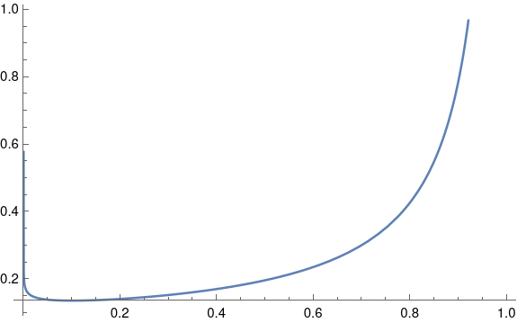
I was thinking about all this yesterday because I was working on a project where the client believes that a proportion θ is around 0.9. A reasonable choice of prior would be beta(0.9, 0.1). Such a distribution has mean 0.9 and is non-informative, and it would be fine for the use I had in mind.
Non-informative beta priors work well in practice, but they’re a little unsettling if you plot them. You’ll notice that the beta(0.9, 0.1) density has singularities at both ends of the interval [0, 1]. The singularity on the right end isn’t so bad, but it’s curious that a distribution designed to have mean 0.9 has infinite density at 0.
If you went further and used a completely non-informative, improper beta(0, 0) prior, you’d have strong singularities at both ends of the interval. And yet this isn’t a problem in practice. Statistical operations that are not expressed in Bayesian terms are often equivalent to a Bayesian analysis with an improper prior like this.
This raises two questions. Why must a non-informative prior put infinite density somewhere, and why is this not a problem?
Beta densities with small parameters have singularities because that’s just the limitation of the beta family. If you were using a strictly subjective Bayesian framework, you would have to say that such densities don’t match anyone’s subjective priors. But the beta distribution is very convenient to use, as explained at the top of this post, and so everyone makes a little ideological compromise.
As for why singular priors are not a problem, it boils down to the difference between density and mass. A beta(0.9, 0.1) distribution has infinite density at 0, but it doesn’t put much mass at 0. If you integrate the density over a small interval, you get a small probability. The singularity on the left is hard to see in the plot above, almost a vertical line that overlaps the vertical axis. So despite the curve going vertical, there isn’t much area under that part of the curve.
You can’t always get what you want. But sometimes you get what you need.