Imagine you picked up a dictionary and found that the pages with A’s were dirty and the Z’s were clean. In between there was a gradual transition with the pages becoming cleaner as you progressed through the alphabet. You might conclude that people have been looking up a lot of words that begin with letters near the beginning of the alphabet and not many near the end.
That’s what Simon Newcomb did in 1881, only he was looking at tables of logarithms. He concluded that people were most interested in looking up the logarithms of numbers that began with 1 and progressively less interested in logarithms of numbers beginning with larger digits. This sounds absolutely bizarre, but he was right. The pattern he described has been repeatedly observed and is called Benford’s law. (Benford re-discovered the same principle in 1938, and per Stigler’s law, Newcomb’s observation was named after Benford.)
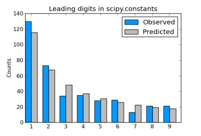
Benford’s law predicts that for data sets such as collections of physical constants, about 30% of the numbers will begin with 1 down to about 5% starting with 8 or 9. To be precise, it says the leading digit will be d with probability log10(1 + 1/d). For a good explanation of Benford’s law, see TAOCP volume 2.
A couple days ago I blogged about using SciPy’s collection of physical constants to look for values that were approximately factorials. Let’s look at that set of constants again and see whether the most significant digits of these constants follows Benford’s law.
Here’s a bar chart comparing the actual number of constants starting with each digit to the results we would expect from Benford’s law.
Here’s the code that was used to create the data for the chart.
from math import log10, floor
from scipy.constants import codata

def most_significant_digit(x):
    e = floor(log10(x))
    return int(x*10**-e)

# count how many constants have each leading digit
count = [0]*10
d = codata.physical_constants
for c in d:
    (value, unit, uncertainty) = d[ c ]
    x = abs(value)
    count[ most_significant_digit(x) ] += 1
total = sum(count)

# expected number of each leading digit per Benford's law
benford = [total*log10(1 + 1./i) for i in range(1, 10)]
The chart itself was produced using matplotlib, starting with this sample code.
The actual counts we see in scipy.constants line up fairly well with the predictions from Benford’s law. The results are much closer to Benford’s prediction than to the uniform distribution that you might have expected before hearing of Benford’s law.
Update: See the next post for an explanation of why factorials also follow Benford’s law.