Robustness and tests for equal variance

The two-sample t-test is a way to test whether two data sets come from distributions with the same mean. I wrote a few days ago about how the test performs under ideal circumstances, as well as less than ideal circumstances.

This is an analogous post for testing whether two data sets come from distributions with the same variance. Statistics texts books often present the F-test for this task, then warn in a footnote that the test is highly dependent on the assumption that both data sets come from normal distributions.

Sensitivity and robustness

Statistics texts give too little attention to robustness in my opinion. Modeling assumptions never hold exactly, so it’s important to know how procedures perform when assumptions don’t hold exactly. Since the F-test is one of the rare instances where textbooks warn about a lack of robustness, I expected the F-test to perform terribly under simulation, relative to its recommended alternatives Bartlett’s test and Levene’s test. That’s not exactly what I found.

Simulation design

For my simulations I selected 35 samples from each of two distributions. I selected significance levels for the F-test, Bartlett’s test, and Levene’s test so that each would have roughly a 5% error rate under a null scenario, both sets of data coming from the same distribution, and a 20% error rate under an alternative scenario.

I chose my initial null and alternative scenarios to use normal (Gaussian) distributions, i.e. to satisfy the assumptions of the F-test. Then I used the same designs for data coming from a fat-tailed distribution to see how well each of the tests performed.

For the normal null scenario, both data sets were drawn from a normal distribution with mean 0 and standard deviation 15. For the normal alternative scenario I used normal distributions with standard deviations 15 and 25.

Normal distribution calibration

Here are the results from the normal distribution simulations.

    |----------+-------+--------+---------|
    | Test     | Alpha | Type I | Type II |
    |----------+-------+--------+---------|
    | F        |  0.13 | 0.0390 |  0.1863 |
    | Bartlett |  0.04 | 0.0396 |  0.1906 |
    | Levene   |  0.06 | 0.0439 |  0.2607 |
    |----------+-------+--------+---------|

Here the Type I column is the proportion of times the test incorrectly concluded that identical distributions had unequal variances. The Type II column reports the proportion of times the test failed to conclude that distributions with different variances indeed had unequal variances. Results were based on simulating 10,000 experiments.

The three tests had roughly equal operating characteristics. The only difference that stands out above simulation noise is that the Levene test had larger Type II error than the other tests when calibrated to have the same Type I error.

To calibrate the operating characteristics, I used alpha levels 0.15, 0.04, and 0.05 respectively for the F, Bartlett, and Levene tests.

Fat-tail simulation results

Next I used the design parameters above, i.e. the alpha levels for each test, but drew data from distributions with a heavier tail. For the null scenario, both data sets were drawn from a Student t distribution with 4 degrees of freedom and scale 15. For the alternative scenario, the scale of one of the distributions was increased to 25. Here are the results, again based on 10,000 simulations.

    |----------+-------+--------+---------|
    | Test     | Alpha | Type I | Type II |
    |----------+-------+--------+---------|
    | F        |  0.13 | 0.2417 |  0.2852 |
    | Bartlett |  0.04 | 0.2165 |  0.2859 |
    | Levene   |  0.06 | 0.0448 |  0.4537 |
    |----------+-------+--------+---------|

The operating characteristics degraded when drawing samples from a fat-tailed distribution, t with 4 degrees of freedom, but they didn’t degrade uniformly.

Compared to the F-test, the Bartlett test had slightly better Type I error and the same Type II error.

The Levene test, had a much lower Type I error than the other tests, hardly higher than it was when drawing from a normal distribution, but had a higher Type II error.

Conclusion: The F-test is indeed sensitive to departures from the Gaussian assumption, but Bartlett’s test doesn’t seem much better in these particular scenarios. Levene’s test, however, does perform better than the F-test, depending on the relative importance you place on Type I and Type II error.

More hypothesis testing posts

Ellipsoid geometry and Haumea

To first approximation, Earth is a sphere. A more accurate description is that the earth is an oblate spheroid, the polar axis being a little shorter than the equatorial diameter. See details here. Other planets are also oblate spheroids as well. Jupiter is further from spherical than the earth is more oblate.

The general equation for the surface of an ellipsoid is

\frac{x^2}{a^2} + \frac{y^2}{b^2} + \frac{z^2}{c^2} = 1

An ellipsoid has three semi-axes: ab, and c. For a sphere, all three are equal to the radius. For a spheroid, two are equal. In an oblate spheroid, like Earth and Jupiter, abc. For a prolate spheroid like Saturn’s moon Enceladus, abc.

Artists conception of Haumea

The dwarf planet Haumea is far from spherical. It’s not even a spheroid. It’s a general (tri-axial) ellipsoid, with a, b, and c being quite distinct. It’s three semi-axes are approximately 1000, 750, and 500 kilometers. The dimensions are not known very accurately. The image above is an artists conception of Haumea and its ring, via Astronomy Picture of the Day.

This post explains how to compute the volume and surface area of an ellipsoid. See that post for details. Here we’ll just copy the Python code from that post.

    from math import sin, cos, acos, sqrt, pi
    from scipy.special import ellipkinc, ellipeinc
    
    def volume(a, b, c):
        return 4*pi*a*b*c/3
    
    def area(a, b, c):
        phi = acos(c/a)
        k = a*sqrt(b**2 - c**2)/(b*sqrt(a**2 - c**2))
        E = ellipeinc(phi, k)
        F = ellipkinc(phi, k)
        elliptic = E*sin(phi)**2 + F*cos(phi)**2
        return 2.0*pi*c**2 + 2*pi*a*b*elliptic/sin(phi)
    
    a, b, c = 1000, 750, 500
    
    print(volume(a, b, c))
    print(area(a, b, c))

Related post: Planets evenly spaced on a log scale

Two-sample t-test and robustness

A two-sample t-test is intended to determine whether there’s evidence that two samples have come from distributions with different means. The test assumes that both samples come from normal distributions.

Robust to non-normality, not to asymmetry

It is fairly well known that the t-test is robust to departures from a normal distribution, as long as the actual distribution is symmetric. That is, the test works more or less as advertised as long as the distribution is symmetric like a normal distribution, but it may not work as expected if the distribution is asymmetric.

This post will explore the robustness of the t-test via simulation. How far can you be from a normal distribution and still do OK? Can you have any distribution as long as it’s symmetric? Does a little asymmetry ruin everything? If something does go wrong, how does it go wrong?

Experiment design

For the purposes of this post, we’ll compare the null hypothesis that two groups both have mean 100 to the alternative hypothesis that one group has mean 100 and the other has mean 110. We’ll assume both distributions have a standard deviation of 15. There is a variation on the two-sample t-test that does not assume equal variance, but for simplicity we will keep the variance the same in both groups.

We’ll do a typical design, 0.05 significance and 0.80 power. That is, under the null hypothesis, that is if the two groups do come from the same distribution, we expect the test to wrongly conclude that the two distributions are different 5% of the time. And under the alternative hypothesis, when the groups do come from distributions with means 100 and 110, we expect the test to conclude that the two means are indeed different 80% of the time.

Under these assumptions, you’d need a sample of 36 in each group.

Python simulation code

Here’s the code we’ll use for our simulation.

    from scipy.stats import norm, t, gamma, uniform, ttest_ind

    num_per_group = 36

    def simulate_trials(num_trials, group1, group2):
        num_reject = 0
        for _ in range(num_trials):
            a = group1.rvs(num_per_group)
            b = group2.rvs(num_per_group)
            stat, pvalue = ttest_ind(a, b)
            if pvalue < 0.05:
                num_reject += 1
        return(num_reject)

Normal simulation

Normal distributions

Let’s see how the two-sample t-test works under ideal conditions by simulating from the normal distributions that the method assumes.

First we simulate from the null, i.e. we draw the data for both groups from the same distribution

    n1 = norm(100, 15)
    n2 = norm(100, 15)
    print( simulate_trials(1000, n1, n2) )

Out of 1000 experiment simulations, the method rejected the null 54 times, very close to the expected number of 50 based on 0.05 significance.

Next we simulate under the alternative, i.e. we draw data from different distributions.

    n1 = norm(100, 15)
    n2 = norm(110, 15)
    print( simulate_trials(1000, n1, n2) )

This time the method rejected the null 804 times in 1000 simulations, very close to the expected 80% based on the power.

Gamma simulation

Gamma distributions

Next we draw data from a gamma distribution. First we draw both groups from a gamma distribution with mean 100 and standard deviation 15. This requires a shape parameter of 44.44 and a scale of 2.25.

    g1 = gamma(a = 44.44, scale=2.25)
    g2 = gamma(a = 44.44, scale=2.25)
    print( simulate_trials(1000, g1, g2) )

Under the null simulation, we rejected the null 64 times out of 1000 simulations, higher than expected, but not that remarkable.

Under the alternative simulation, we pick the second gamma distribution to have mean 110 and standard deviation 15, which requires shape 53.77 and scale 2.025.

    g1 = gamma(a = 44.44, scale=2.25)
    g2 = gamma(a = 53.77, scale=2.045)
    print( simulate_trials(1000, g1, g2) )

We rejected the null 805 times in 1000 simulations, in line with what you’d expect from the power.

Gamma distributions

When the gamma distribution has such large shape parameters, the distributions are approximately normal, though slightly asymmetric. To increase the asymmetry, we’ll use a couple gamma distributions with smaller mean but shifted over to the right. Under the null, we create two gamma distributions with mean 10 and standard deviation 15, then shift them to the right by 90.

    g1 = gamma(a = 6.67, scale=1.5, loc=90)
    g2 = gamma(a = 6.67, scale=1.5, loc=90)
    print( simulate_trials(1000, g1, g2) )

Under this simulation we reject the null 56 times out of 1000 simulations, in line with what you’d expect.

For the alternative simulation, we pick the second distribution to have a mean of 20 and standard deviation 15, and then shift it to the right by 90 so tht it has mean 110. This distribution has quite a long tail.

    g1 = gamma(a = 6.67, scale=1.5, loc=90)
    g2 = gamma(a = 1.28, scale=11.25, loc=90)
    print( simulate_trials(1000, g1, g2) )

This time we rejected the null 499 times in 1000 simulations. This is a serious departure from what’s expected. Under the alternative hypothesis, we reject the null 50% of the time rather than the 80% we’d expect. If higher mean is better, this means that half the time you’d fail to conclude that the better group really is better.

Uniform distribution simulation

Next we use uniform random samples from the interval [74, 126]. This is a symmetric distribution with mean 100 and standard deviation 15. When we draw both groups from this distribution we rejected the null 48 times, in line with what we’d expect.

    u1 = uniform(loc=74, scale=52)
    u2 = uniform(loc=74, scale=52)
    print( simulate_trials(1000, u1, u2) )

If we move the second distribution over by 10, drawing from [84, 136], we rejected the null 790 times out of 1000, again in line with what you’d get from a normal distribution.

    u1 = uniform(loc=74, scale=52)
    u2 = uniform(loc=84, scale=52)
    print( simulate_trials(1000, u1, u2) )

In this case, we’ve made a big departure from normality and the test still worked as expected. But that’s not always the case, as in the t(3) distribution below.

Student-t simulation (fat tails)

Finally we simulate from a Student-t distribution. This is a symmetric distribution but it has fat tails relative to the normal distribution.

t distributions with 6 dof

First, we simulate from a t distribution with 6 degrees of freedom and scale 12.25, making the standard deviation 15. We shift the location of the distribution by 100 to make the mean 100.

    t1 = t(df=6, loc=100, scale=12.25)
    t2 = t(df=6, loc=100, scale=12.25)
    print( simulate_trials(1000, t1, t2) )

When both groups come from this distribution, we rejected the null 46 times. When we shifted the second distribution to have mean 110, we rejected the null 777 times out of 1000.

    t1 = t(df=6, loc=100, scale=12.25)
    t2 = t(df=6, loc=110, scale=12.25)
    print( simulate_trials(1000, t1, t2) )

In both cases, the results are in line what we’d expect given a 5% significance level and 80% power.

t distributions with 3 dof

A t distribution with 6 degrees of freedom has a heavy tail compared to a normal. Let’s try making the tail even heavier by using 3 degrees of freedom. We make the scale 15 to keep the standard deviation at 15.

    t1 = t(df=3, loc=100, scale=15)
    t2 = t(df=3, loc=100, scale=15)
    print( simulate_trials(1000, t1, t2) )

When we draw both samples from the same distribution, we rejected the null 37 times out of 1000, less than the 50 times we’d expect.

    t1 = t(df=3, loc=100, scale=15)
    t2 = t(df=3, loc=110, scale=15)
    print( simulate_trials(1000, t1, t2) )

When we shift the second distribution over to have mean 110, we rejected the null 463 times out of 1000, far less than the 80% rejection you’d expect if the data were normally distributed.

Just looking at a plot of the PDFs, a t(3) looks much closer to a normal distribution than a uniform distribution does. But the tail behavior is different. The tails of the uniform are as thin as you can get—they’re zero!—while the t(3) has heavy tails.

These two examples show that you can replace the normal distribution with a moderately heavy tailed symmetric distribution, but don’t overdo it. When the data some from a heavy tailed distribution, even one that is symmetric, the two-sample t-test may not have the operating characteristics you’d expect.

Spectral sparsification

The latest episode of My Favorite theorem features John Urschel, former offensive lineman for the Baltimore Ravens and current math graduate student. His favorite theorem is a result on graph approximation: for every weighted graph, no matter how densely connected, it is possible to find a sparse graph whose Laplacian approximates that of the original graph. For details see Spectral Sparsification of Graphs by Dan Spielman and Shang-Hua Teng.

You could view this theorem as a positive result—it’s possible to find good sparse approximations—or a negative result—the Laplacian doesn’t capture very well how densely a graph is connected.

Related: Blog posts based on my interview with Dan Spielman at the 2014 Heidelberg Laureate Forum.

Reciprocals of primes

Here’s an interesting little tidbit:

For any prime p except 2 and 5, the decimal expansion of 1/p repeats with a period that divides p − 1.

The period could be as large as p − 1, but no larger. If it’s less than p − 1, then it’s a divisor of p − 1.

Here are a few examples.

1/3 = 0.33…
1/7 = 0.142857142857…
1/11= 0.0909…
1/13 = 0.076923076923…
1/17 = 0.05882352941176470588235294117647…
1/19 = 0.052631578947368421052631578947368421…
1/23 = 0.04347826086956521739130434782608695652173913…

Here’s a table summarizing the periods above.

|-------+--------|
| prime | period |
|-------+--------|
|     3 |      1 |
|     7 |      6 |
|    11 |      2 |
|    13 |      6 |
|    17 |     16 |
|    19 |     18 |
|    23 |     22 |
|-------+--------|

For a proof of the claims above, and more general results, see Periods of Fractions.

Rise and fall of the Windows Empire

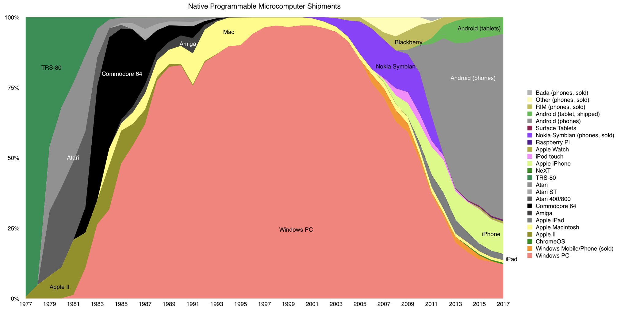
This morning I ran across the following graph via Horace Dediu.

Computer market share

I developed Windows software during the fattest part of the Windows curve. That was a great time to be in the Windows ecosystem.

Before that I was in an academic bubble. My world consisted primarily of Macs and various flavors of Unix. I had no idea that my world was a tiny minority. I had a PC at home, but mostly used it as a terminal to connect to remote Unix machines, and didn’t realize that Windows was so dominant.

When I found out I’d been very wrong in my perception of market share, I determined not to be naive again. Ever since then I regularly look around to keep an eye on the landscape.

The graph above combines desktop and mobile computers, and you may or may not think that’s appropriate. Relative to the desktop market, Windows remains dominant, but the desktop market share itself has shrunk, not so much in absolute size but relative to total computer market.

Last time I looked, about 70% of the traffic to this website comes from desktops. I still consider the desktop the place for “real work,” and many people feel the same way.

It’s conventional to say the Roman Empire fell in 476 AD, but this would have been a surprise to those living in the eastern half of the empire who considered themselves to be Roman. The eastern (Byzantine) empire continued for another thousand years after the western empire fell.

The Windows empire hasn’t fallen, but has changed. Microsoft is doing well, as far as I know. I don’t keep up with Microsoft as much as I used to. I have no animosity toward Microsoft, but I’m no longer doing the kind of work their tools are intended for. I still use Windows—I’m writing this blog post from my Windows 10 machine—though I also use Mac, Linux, iOS, and Android.


Robust statistics

P. J. Huber gives three desiderata for a statistical method in his book Robust Statistics:

  1. It should have a reasonably good (optimal or nearly optimal) efficiency at the assumed model.
  2. It should be robust in the sense that small deviations from the model assumptions should impair the performance only slightly.
  3. Somewhat larger deviations from the model should not cause a catastrophe.

Robust statistical methods are those that strive for these properties. These are not objective properties per se though there are objective ways to try to quantify robustness in various contexts.

(In Nassim Taleb’s tricotomy of fragile, robust, and anti-fragile, robustness is in the middle. Something is fragile if it is harmed by volatility, and anti-fragile if it benefits from volatility. Robustness is in the middle. It is not unduly harmed by volatility, but does not benefit from it either. In the context of statistical methods, volatility is departure from modeling assumptions. Hardly anything benefits from modeling assumptions being violated, but some methods are harmed by such violations more or less than others.)

Here are several blog posts I’ve written about robustness:

Optimal low-rank matrix approximation

Matrix compression

Suppose you have an m by n matrix A, where m and n are very large, that you’d like to compress. That is, you’d like to come up with an approximation of A that takes less data to describe.

For example, consider a high resolution photo that as a matrix of gray scale values. An approximation to the matrix could be a lower resolution representation that takes less space.

I heard a rumor many years ago that space probes would compress images by interpreting an image as a matrix and sending back a few eigenvalues and eigenvectors. That sounded fascinating, but what about images that aren’t square? If a matrix M is not square, then you can’t have Mx = λx for a scalar λ because the left and right sides of the equation would have different dimensions.

Truncated SVD

Approximate a rectangular matrix requires using something more general than eigenvalues and eigenvectors, and that is singular values and singular vectors.

Suppose our matrix A has the singular value decomposition

A = U \Sigma V^*

This can be written as

A = \sum_{i=1}^p \sigma_i u_i v_i^*

where the σi are the singular values and p is the number of singular values that are non-zero. The ui and vi are the ith columns of U and V respectively. Singular values are nonnegative, and listed in decreasing order.

We can form an approximation to A by truncating the sum above. Instead of taking all the singular values, and their corresponding left and right singular vectors, we only take the k largest singular values and their corresponding vectors.

A_k = \sum_{i=1}^k \sigma_i u_i v_i^*

This is called the truncated SVD.

We started by assuming A had dimensions m by n and that both were large. Storing A requires mn numbers. Storing Ak requires only k(1 + mn) numbers. This is a big savings if k is much smaller than m and n.

Eckart-Young theorem

So how good an approximation is Ak ? Turns out it is optimal, in the least squares sense. This is the content of the Eckart-Young theorem. It says that the best least squares (2-norm) approximation of A by a rank k matrix is given by Ak.

Not only that, the theorem says the 2-norm error is given by the first singular value that we didn’t use, i.e.

|| A - A_k ||_2 = \sigma_{k+1}

More linear algebra posts

Least squares solutions to over- or underdetermined systems

If often happens in applications that a linear system of equations Axb either does not have a solution or has infinitely many solutions. Applications often use least squares to create a problem that has a unique solution.

Overdetermined systems

Suppose the matrix A has dimensions m by n and the right hand side vector b has dimension m. Then the solution x, if it exists, has to have dimension n. If mn, i.e. we have more equations than unknowns, the system is overdetermined. The equations will be inconsistent in general. This is typical, for example, in linear regression.

In this case, you can use the least square criterion to determine a solution. Instead of demanding that Axb, we look for an x than makes the difference between Ax and b as small as possible, as measured by the 2-norm (root mean square). That is, we pick x to minimize

|| Ax - b||_2^2

meaning we solve the system as best we can, best as measured by the 2-norm.

Underdetermined systems

If the number of rows in the matrix A, i.e. the number of equations, is less than the number of columns, i.e. the number of unknowns, then the system is underdetermined. In general there were be infinitely many solutions. It’s also possible that there are no solutions because the equations are inconsistent.

In this case, we can use least squares to assure that a solution exists, and to decide which of the many possible solutions to choose. Here we want to find the x that minimizes

|| Ax - b ||_2^2 + ||x||_2^2

If there are values of x that satisfy Axb then this will chose the solution with least norm.

Least squares solutions and SVD

If the singular value decomposition (SVD) of a real matrix A is given by

A = U \Sigma V^T
and A has rank r, then the least squares solution to the system Axb is given explicitly by

x = \sum_{i=1}^r \frac{u_i^T b}{\sigma_i} v_i

where the u‘s are the columns of U and the v‘s are the columns of v.

Note that the denominators are not zero; the fact that A has rank r means that it has r positive singular values.

Furthermore, the least squares residual, i.e. the degree to which Ax differs from b, is given by

||Ax -b ||_2^2 = \sum_{i = r+1}^m (u_i^Tb)^2

Note that if the matrix A has rank m, then the least squares problem can be solved exactly, and the right side above is an empty sum.

See, for example, Golub and Van Loan’s classic book Matrix Computations.

More linear algebra posts

Computing SVD and pseudoinverse

In a nutshell, given the singular decomposition of a matrix A,

A = U \Sigma V^*

the Moore-Penrose pseudoinverse is given by

A^+ = V \Sigma^+ U^*.

This post will explain what the terms above mean, and how to compute them in Python and in Mathematica.

Singular Value Decomposition (SVD)

The singular value decomposition of a matrix is a sort of change of coordinates that makes the matrix simple, a generalization of diagonalization.

Matrix diagonalization

If a square matrix A is diagonalizable, then there is a matrix P such that

A = P D P^{-1}

where the matrix D is diagonal. You could think of P as a change of coordinates that makes the action of A as simple as possible. The elements on the diagonal of D are the eigenvalues of A and the columns of P are the corresponding eigenvectors.

Unfortunately not all matrices can be diagonalized. Singular value decomposition is a way to do something like diagonalization for any matrix, even non-square matrices.

Generalization to SVD

Singular value decomposition generalizes diagonalization. The matrix Σ in SVD is analogous to D in diagonalization. Σ is diagonal, though it may not be square. The matrices on either side of Σ are analogous to the matrix P in diagonalization, though now there are two different matrices, and they are not necessarily inverses of each other. The matrices U and V are square, but not necessarily of the same dimension.

The elements along the diagonal of Σ are not necessarily eigenvalues but singular values, which are a generalization of eigenvalues. Similarly the columns of U and V are not necessarily eigenvectors but left singular vectors and right singular vectors respectively.

The star superscript indicates conjugate transpose. If a matrix has all real components, then the conjugate transpose is just the transpose. But if the matrix has complex entries, you take the conjugate and transpose each entry.

The matrices U and V are unitary. A matrix M is unitary if its inverse is its conjugate transpose, i.e. M* M = MM* = I.

Pseudoinverse and SVD

The (Moore-Penrose) pseudoinverse of a matrix generalizes the notion of an inverse, somewhat like the way SVD generalized diagonalization. Not every matrix has an inverse, but every matrix has a pseudoinverse, even non-square matrices.

Computing the pseudoinverse from the SVD is simple.

If

A = U \Sigma V^*

then

A^+ = V \Sigma^+ U^*

where Σ+ is formed from Σ by taking the reciprocal of all the non-zero elements, leaving all the zeros alone, and making the matrix the right shape: if Σ is an m by n matrix, then Σ+ must be an n by m matrix.

We’ll give examples below in Mathematica and Python.

Computing SVD in Mathematica

Let’s start with the matrix A below.

A = \begin{bmatrix} 2 & -1 & 0 \\ 4 & 3 & -2 \end{bmatrix}

We can find the SVD of A with the following Mathematica commands.

    A = {{2, -1, 0}, {4, 3, -2}}
    {U, S, V} = SingularValueDecomposition[A]

From this we learn that the singular value decomposition of A is

\begin{bmatrix} \frac{1}{\sqrt{26}} & -\frac{5}{\sqrt{26}} \\ \frac{5}{\sqrt{26}} & \frac{1}{\sqrt{26}} \\ \end{bmatrix} \begin{bmatrix} \sqrt{30} & 0 & 0 \\ 0 & 2 & 0 \end{bmatrix} \begin{bmatrix} \frac{11}{\sqrt{195}} & \frac{7}{\sqrt{195}} & -\sqrt{\frac{5}{39}} \\ -\frac{3}{\sqrt{26}} & 2 \sqrt{\frac{2}{13}} & -\frac{1}{\sqrt{26}} \\ \frac{1}{\sqrt{30}} & \sqrt{\frac{2}{15}} & \sqrt{\frac{5}{6}} \end{bmatrix}

Note that the last matrix is not V but the transpose of V. Mathematica returns V itself, not its transpose.

If we multiply the matrices back together we can verify that we get A back.

    U . S. Transpose[V]

This returns

    {{2, -1, 0}, {4, 3, -2}}

as we’d expect.

Computing pseudoinverse in Mathematica

The Mathematica command for computing the pseudoinverse is simply PseudoInverse. (The best thing about Mathematica is it’s consistent, predictable naming.)

    PseudoInverse[A]

This returns

    {{19/60, 1/12}, {-(11/30), 1/6}, {1/12, -(1/12)}}

And we can confirm that computing the pseudoinverse via the SVD

    Sp = {{1/Sqrt[30], 0}, {0, 1/2}, {0, 0}}
    V . Sp . Transpose[U]

gives the same result.

Computing SVD in Python

Next we compute the singular value decomposition in Python (NumPy).

    >>> a = np.matrix([[2, -1, 0],[4,3,-2]])
    >>> u, s, vt = np.linalg.svd(a, full_matrices=True)

Note that np.linalg.svd returns the transpose of V, not the V in the definition of singular value decomposition.

Also, the object s is not the diagonal matrix Σ but a vector containing only the diagonal elements, i.e. just the singular values. This can save a lot of space if the matrix is large. The NumPy method svd has other efficiency-related options that I won’t go into here.

We can verify that the SVD is correct by turning s back into a matrix and multiply the components together.

    >>> ss = np.matrix([[s[0], 0, 0], [0, s[1], 0]])
    >>> u*ss*vt

This returns the matrix A, within floating point accuracy. Since Python is doing floating point computations, not symbolic calculation like Mathematica, the zero in A turns into -3.8e-16.

Note that the singular value decompositions as computed by Mathematica and Python differ in a few signs here and there; the SVD is not unique.

Computing pseudoinverse in Python

The pseudoinverse can be computed in NumPy with np.linalg.pinv.

    >>> np.linalg.pinv(a)
    matrix([[ 0.31666667,  0.08333333],
            [-0.36666667,  0.16666667],
            [ 0.08333333, -0.08333333]])

This returns the same result as Mathematica above, up to floating point precision.

More linear algebra posts