Goldbach’s conjecture, Lagrange’s theorem, and 2019

The previous post showed how to find all groups whose order is a product of two primes using 2019 as an example. Here are a couple more observations along the same line, illustrating the odd Goldbach conjecture and Lagrange’s four-square theorem with 2019.

Odd Goldbach Conjecture

Goldbach’s conjecture says that every even number greater than 2 can be written as the sum of two primes. The odd Goldbach conjecture, a.k.a. the weak Goldbach conjecture, says that every odd number greater than 5 can be written as the sum of three primes. The odd Goldbach conjecture isn’t really a conjecture anymore because Harald Helfgott proved it in 2013, though the original Goldbach conjecture remains unsettled.

The odd Goldbach conjecture says it should be possible to write 2019 as the sum of three primes. And in fact there are 2,259 ways to write 2019 as a non-decreasing sequence of primes.

      3 +   5 + 2011
      3 +  13 + 2003
      3 +  17 + 1999
          ...
    659 + 659 +  701
    659 + 677 +  701
    673 + 673 +  673

Lagrange’s four-square theorem

Lagrange’s four-square theorem says that every non-negative integer can be written as the sum of four squares. 2019 is a non-negative integer, so it can be written as the sum of four squares. In fact there are 66 ways to write 2019 as a sum of four squares.

     0  1 13 43
     0  5 25 37
     0  7 11 43
         ...
    16 19 21 31
    17 23 24 25
    19 20 23 27

Sometimes there is a unique way to write a number as the sum of four squares. The last time a year could be written uniquely as a sum of four squares was 1536, and the next time will be in 2048.

Related posts

Groups of order 2019

How many groups have 2019 elements? What are these groups?

2019 is a semiprime, i.e. the product of two primes, 3 and 673. For every semiprime s, there are either one or two distinct groups of order s.

As explained here, if spq with pq, all groups of order s are isomorphic if q is not a factor of p − 1. If q does divide p − 1 then there are exactly two non-isomorphic groups of order s, one abelian and one non-abelian. In our case, 3 does divide 672, so there are two groups of order 2019. The first is easy: the cyclic group of order 2019. The second is more complex.

You could take the direct product of the cyclic groups of order 3 and 673, but that turns out to be isomorphic to the cyclic group of order 2019. But if you take the semidirect product you get the other group of order 2019, the non-abelian one.

Semidirect products

Starting with two groups G and H, the direct product G × H is the Cartesian product of G and H with multiplication defined componentwise. The semidirect product of G and H, written [1]

G \rtimes H

also starts with the Cartesian product of G and H but defines multiplication differently.

In our application, G will be the integers mod 673 with addition and H will be a three-element subgroup of the integers mod 673 with multiplication [2]. Let H be the set {1, 255, 417} with respect to multiplication [3]. Note that 1 is its own inverse and 255 and 417 are inverses of each other.

Product

Now the group product of (g1, h1) and (g2, h2) is defined to be

(g1 + h1−1g2, h1 h2)

So, for example, the product of (5, 255) and (334, 417) is (5 + 417*334, 255*417) which reduces to (645, 1) working mod 673.

(We haven’t defined the semidirect product in general, but the procedure above suffices to define the semidirect product for any two groups of prime order, and so it is sufficient to find all groups of semiprime order.)

Note that our group is non-abelian. For example, if we reverse the order of multiplication above we get (263, 1).

Identity

The identity element is just the pair consisting of the identity elements from G and H. In our case, this is (0, 1) because 0 is the additive identity and 1 is the multiplicative identity.

Inverse

The inverse of an element (gh) is given by

(−ghh−1).

So, for example, the inverse of (600, 255) is (444, 417).

Python code

The goal of this post is to be concrete rather than general.

So to make everything perfectly explicit, we’ll write a little Python code implementing the product and inverse.

    
    def hinv(h):
        if h == 255:
            return 417
        if h == 417:
            return 255
        if h == 1:
            return 1
    
    def prod(x, y):
        g1, h1 = x
        g2, h2 = y
        g3 = (g1 + hinv(h1)*g2) % 673
        h3 = (h1*h2) % 673
        return (g3, h3)
    
    def group_inv(x):
        g, h = x
        return ((-g*h)%673, hinv(h))
    
    x = (5, 255)
    y = (334, 417)
    print(prod(x, y))
    print(prod(y, x))
    print(group_inv((600, 255)))

The following code verifies that our group satisfies the axioms of a group.

    from itertools import product
    
    identity = (0, 1)
    h_list = [1, 255, 417]
    
    def elem(x):
        g, h = x
        g_ok = (0 <= g <= 672)
        h_ok = (h in h_list)
        return (g_ok and h_ok)
    
    group = product(range(673), h_list)
    assert(len([g for g in group]) == 2019)
    
    # closed under multiplication    
    for x in group:
        for y in group:
            assert( elem(prod(x, y)) )
    
    # multiplication is associative
    for x in group:
        for y in group:
            for z in group:
                xy_z = prod(prod(x, y),z)
                x_yz = prod(x, prod(y,z))
                assert(xy_z == x_yz)
    
    # identity acts like it's supposed to
    for x in group:
        assert( prod(x, identity) == x )
        assert( prod(identity, x) == x )
    
    # every element has an inverse
    for x in group:
        ginv = group_inv(x)
        assert( elem(ginv) )
        assert( prod(x, ginv) == identity )
        assert( prod(ginv, x) == identity )

Related posts

[1] The symbol for semidirect product is ⋊. It’s U+22CA in Unicode and \rtimes in LaTeX.

[2] In general, the semidirect product depends on a choice of an action of the group H on the group G. Here the action is multiplication by an element of H. Different actions can result in different groups. Sometimes the particular choice of action is made explicit as a subscript on the ⋊ symbol.

[3] How did I find these numbers? There are 672 non-zero numbers mod 673, so I picked a number, it happened to be 5, and raised it to the powers 672/3 and 2*672/3.

 

Flattest US states

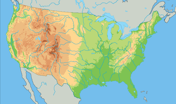
US physical map

I read somewhere that, contrary to popular belief, Kansas is not the flattest state in the US. Instead, Florida is the flattest, and Kansas was several notches further down the list.

(Update: Nevertheless, Kansas is literally flatter than a pancake. Thanks to Andreas Krause for the link in the comments.)

How would you measure the flatness of a geographic region? The simplest approach would be to look at the range of elevation from the highest point to the lowest point, so that’s what I did. Here are elevations and differences for each state, measured in feet.

|----------------+-------+------+-------|
| State          |  High |  Low |  Diff |
|----------------+-------+------+-------|
| Florida        |   345 |    0 |   345 |
| Delaware       |   450 |    0 |   450 |
| Louisiana      |   535 |   -7 |   542 |
| Mississippi    |   807 |    0 |   807 |
| Rhode Island   |   814 |    0 |   814 |
| Indiana        |  1257 |  322 |   935 |
| Illinois       |  1237 |  279 |   958 |
| Ohio           |  1549 |  456 |  1093 |
| Iowa           |  1670 |  479 |  1191 |
| Wisconsin      |  1952 |  581 |  1371 |
| Michigan       |  1982 |  571 |  1411 |
| Missouri       |  1772 |  230 |  1542 |
| Minnesota      |  2303 |  600 |  1703 |
| New Jersey     |  1804 |    0 |  1804 |
| Connecticut    |  2382 |    0 |  2382 |
| Alabama        |  2405 |    0 |  2405 |
| Arkansas       |  2756 |   56 |  2700 |
| North Dakota   |  3507 |  751 |  2756 |
| Pennsylvania   |  3215 |    0 |  3215 |
| Kansas         |  4042 |  679 |  3363 |
| Maryland       |  3363 |    0 |  3363 |
| Massachusetts  |  3491 |    0 |  3491 |
| South Carolina |  3563 |    0 |  3563 |
| Kentucky       |  4144 |  256 |  3888 |
| Vermont        |  4396 |   95 |  4301 |
| Nebraska       |  5427 |  840 |  4587 |
| West Virginia  |  4865 |  240 |  4625 |
| Oklahoma       |  4977 |  289 |  4688 |
| Georgia        |  4787 |    0 |  4787 |
| Maine          |  5269 |    0 |  5269 |
| New York       |  5348 |    0 |  5348 |
| Virginia       |  5732 |    0 |  5732 |
| South Dakota   |  7247 |  968 |  6279 |
| New Hampshire  |  6293 |    0 |  6293 |
| Tennessee      |  6647 |  177 |  6470 |
| North Carolina |  6690 |    0 |  6690 |
| Texas          |  8753 |    0 |  8753 |
| New Mexico     | 13169 | 2844 | 10325 |
| Wyoming        | 13812 | 3100 | 10712 |
| Montana        | 12808 | 1801 | 11007 |
| Colorado       | 14439 | 3314 | 11125 |
| Oregon         | 11247 |    0 | 11247 |
| Utah           | 13527 | 2001 | 11526 |
| Idaho          | 12667 |  712 | 11955 |
| Arizona        | 12631 |   69 | 12562 |
| Nevada         | 13146 |  479 | 12667 |
| Hawaii         | 13806 |    0 | 13806 |
| Washington     | 14419 |    0 | 14419 |
| California     | 14505 | -282 | 14787 |
| Alaska         | 20335 |    0 | 20335 |
|----------------+-------+------+-------|

By the measure used in the table above, Florida is about 10 times flatter than Kansas.

The centroid of the continental US is in Kansas, and if you look at the center of the map above, you’ll see that there’s an elevation change across Kansas.

If I remember correctly, the source I saw said that Kansas was something like 9th, though in the table above it is 20th. Maybe that source measured flatness differently. If you had a grid of measurements throughout each state, you could compute something like a Sobolev norm that accounts for gradients.

Naked eye view vs photos of the northern lights

My daughter Elizabeth recently photographed the northern lights (aurora borealis) in Tromsø, Norway, about 3° above the Arctic Circle.

Northern lights, Tromsøm 2018

I haven’t seen the northern lights in person, and I didn’t know until she told me that the lights appear gray to the naked eye, like smoke. Sometimes the lights have a hint of color, but the color is nowhere near as intense as in photographs. Photos like the one above are not false color images. The green light is really there, even though it is not nearly as vivid to the naked eye as it is to a camera.

The reason the aurora appear gray is that human eyes don’t see in color well in dim light. At very low light levels, our vision is based entirely on rods, photoreceptor cells that are very sensitive to light but not to color. If aurora are bright enough, cones are activated and color becomes visible.

Why green in particular? It comes from excited oxygen atoms, emitting radiation at a wavelength of 557.7 nm. Other colors can be found in aurora, but green is most common for physical and physiological reasons. The physical reasons involve radiation and the chemical composition of the atmosphere. The physiological reason is that human vision is most sensitive around the frequency of green light.

Related posts

Check sums and error detection

The previous post looked at Crockford’s base 32 encoding, a minor variation on the way math conventionally represents base 32 numbers, with concessions for human use. By not using the letter O, for example, it avoids confusion with the digit 0.

Crockford recommends the following check sum procedure, a simple error detection code:

The check symbol encodes the number modulo 37, 37 being the least prime number greater than 32.

That is, we take the remainder when the base 32 number is divided by 37 and append the result to the original encoded number. The remainder could be larger than 31, so we need to expand our alphabet of symbols. Crockford recommends using the symbols *, ~, $, =, and U to represent remainders of 32, 33, 34, 35, and 36.

Crockford says his check sum will “detect wrong-symbol and transposed-symbol errors.” We will show that this is the case in the proof below.

Python example

Here’s a little Python code to demonstrate how the checksum works

    from base32_crockford import encode, decode

    s = "H88CMK9BVJ1V"
    w = "H88CMK9BVJ1W" # wrong last char
    t = "H88CMK9BVJV1" # transposed last chars

    def append_checksum(s):
        return encode(decode(s), checksum=True)

    print(append_checksum(s))
    print(append_checksum(w))
    print(append_checksum(t))

This produces the following output.

    H88CMK9BVJ1VP
    H88CMK9BVJ1WQ
    H88CMK9BVJV1E

The checksum character of the original string is P. When the last character is changed, the checksum changes from P to Q. Similarly, transposing the last two characters changes the checksum from P to E.

The following code illustrates that the check sum can be a non-alphabetic character.

    s = "H88CMK9BVJ10"
    n = decode(s)
    r = n % 37
    print(r)
    print(encode(n, checksum=True))

This produces

    32
    H88CMK9BVJ10*

As we said above, a remainder of 32 is represented by *.

Proof

If you change one character in a base 32 number, its remainder by 37 will change as well, and so the check sum changes.

Specifically, if you change the nth digit from the right, counting from 0, by an amount k, then you change the number by a factor of k 32n. Since 0 < k < 32, k is not divisible by 37, nor is 32n. Because 37 is prime, k 32n is not divisible by 37 [1]. The same argument holds if we replace 37 by any larger prime.

Now what about transpositions? If you swap consecutive digits a and b in a number, you also change the remainder by 37 (or any larger prime) and hence the check sum.

Again, let’s be specific. Suppose we transpose the nth and (n + 1)st digits from the right, again counting from 0. Denote these digits by a and b respectively. Then swapping these two digits changes the number by an amount

(b 2n+1 + a 2n) − (a 2n+1 + b 2n) = (ba) 2n

If ab, then ba is a number between −31 and 31, but not 0, and so ba is not divisible by 37. Neither is any power of 2 divisible by 37, so we’ve changed the remainder by 37, i.e. changed the check sum. And as before, the same argument works for any prime larger than 47.

Related posts

[1] A prime p divides a product ab only if it divides a or it divides b. This isn’t true for composite numbers. For example, 6 divides 4*9 = 36, but 6 doesn’t divide 4 or 9.

Base 32 and base 64 encoding

Math has a conventional way to represent numbers in bases larger than 10, and software development has a couple variations on this theme that are only incidentally mathematical.

Math convention

By convention, math books typically represent numbers in bases larger than 10 by using letters as new digit symbols following 9. For example, base 16 would use 0, 1, 2, …, 9, A, B, C, D, E, and F as its “digits.” This works for bases up to 36; base 36 would use all the letters of the alphabet. There’s no firm convention for whether to use upper or lower case letters.

Base 64 encoding

The common use for base 64 encoding isn’t to represent bits as numbers per se, but to have an efficient way to transmit bits in a context that requires text characters.

There are around 100 possible characters on a keyboard, and 64 is the largest power of 2 less than 100 [1], and so base 64 is the most dense encoding using common characters in a base that is a power of 2.

Base 64 encoding does not follow the math convention of using the digits first and then adding more symbols; it’s free not to because there’s no intention of treating the output as numbers. Instead, the capital letters A through Z represent the numbers 0 though 25, the lower case letters a through z represent the numbers 26 through 51, and the digits 0 through 9 represent the numbers 52 through 61. The symbol + is used for 62 and / is used for 63.

Crockford’s base 32 encoding

Douglas Crockford proposed an interesting form of base 32 encoding. His encoding mostly follows the math convention: 0, 1, 2, …, 9, A, B, …, except he does not use the letters I, L, O, and U. This eliminates the possibility of confusing i, I, or l with 1, or confusing O with 0. Crockford had one more letter he could eliminate, and he chose U in order to avoid an “accidental obscenity.” [2]

Crockford’s base 32 encoding is a compromise between efficiency and human legibility. It is more efficient than hexadecimal, representing 25% more bits per character. It’s less efficient than base 64, representing 17% fewer bits per character, but is more legible than base 64 encoding because it eliminates commonly confused characters.

His encoding is also case insensitive. He recommends using only capital letters for output, but permitting upper or lower case letters in input. This is in the spirit of Postel’s law, also known as the robustness principle:

Be conservative in what you send, and liberal in what you accept.

See the next post for an explanation of Crockford’s check sum proposal.

A password generator

Here’s a Python script to generate passwords using Crockford’s base 32 encoding.

    from secrets import randbits
    from base32_crockford import encode

    def gen_pwd(numbits):
        print(encode(randbits(numbits)))

For example, gen_pwd(60) would create a 12-character password with 60-bits of entropy, and this password would be free of commonly confused characters.

Related posts

[1] We want to use powers of 2 because it’s easy to convert between base 2 and base 2n: start at the right end and convert bits in groups of n. For example, to convert a binary string to hexadecimal (base 24 = 16), convert groups of four bits each to hexadecimal. So to convert the binary number 101111001 to hex, we break it into 1 0111 1001 and convert each piece to hex, with 1 -> 1, 0111 -> 7, and 1001 -> 9, to find 101111001 -> 179. If we a base that is not a power of 2, the conversion would be more complicated and not so localized.

[2] All the words on George Carlin’s infamous list include either an I or a U, and so none can result from Crockford’s base 32 encoding. If one were willing to risk accidental obscenities, it would be good to put U back in and remove S since the latter resembles 5, particularly in some fonts.

Most popular posts of 2018

Here are 10 of my most popular posts this year, arranged as pairs of posts in different areas.

Astronomy

Programming

Computer arithmetic

Math

Statistics

New prime record: 51st Mersenne prime discovered

A new prime record was announced yesterday. The largest known prime is now

2^{82,589,933} - 1

Written in hexadecimal the newly discovered prime is

1\underbrace{\mbox{FFF \ldots FFF}}_\mbox{{\normalsize 20,647,483 F's}}

For decades the largest known prime has been a Mersenne prime because there’s an efficient test for checking whether a Mersenne number is prime. I explain the test here.

There are now 51 known Mersenne primes. There may be infinitely many Mersenne primes, but this hasn’t been proven. Also, the newly discovered Mersenne prime is the 51st known Mersenne prime, but it may not be the 51st Mersenne prime, i.e. there may be undiscovered Mersenne primes hiding between the last few that have been discovered.

Three weeks ago I wrote a post graphing the trend in Mersenne primes. Here’s the updated post. Mersenne primes have the form 2p − 1 where p is a prime, and this graph plots the values of p on a log scale. See the earlier post for details.

Trend in Mersenne primes

Because there’s a one-to-one correspondence between Mersenne primes and even perfect numbers, the new discovery means there is also a new perfect number. M is a Mersenne prime if and only if M(M + 1)/2 is an even perfect number. This is also the Mth triangular number.

Related posts

Multi-arm adaptively randomized clinical trials

This post will look at adaptively randomized trial designs. In particular, we want to focus on multi-arm trials, i.e. trials of more than two treatments. The aim is to drop the less effective treatments quickly so the trial can focus on determining which of the better treatments is best.

We’ll briefly review our approach to adaptive randomization but not go into much detail. For a more thorough introduction, see, for example, this report.

Why adaptive randomization

Adaptive randomization designs allow the randomization probabilities to change in response to accumulated outcome data so that more subjects are assigned to (what appear to be) more effective treatments. They also allow for continuous monitoring, so one can stop a trial early if we’re sufficiently confident that we’ve found the best treatment.

Adapting randomization probabilities

Of course we don’t know what treatments are more effective or else we wouldn’t be running a clinical trial. We have an idea based on the data seen so far at any point in the trial, and that assessment may change as more data become available.

We could simply put each patient on what appears to be the best arm (the “play-the-winner” strategy), but this would forgo the benefits of randomization. Instead we compromise, continuing to randomize, but increasing the randomization probability for what appears to be the best treatment at the time a subject enters the trial.

Continuous monitoring

By monitoring the performance of each treatment arm, we can drop a poorly performing arm and assign subjects to the better treatment arms. This is particularly important for multi-arm trials. We want to weed out the poor treatments quickly so we can focus on the more promising treatments.

Continuous monitoring opens the possibility of stopping trials early if there is a clear winner. If all treatments perform similarly, more patients will be used. The maximum number of patients will be enrolled only if necessary.

Multi-arm trials

Randomizing an equal number of patients to each of several treatment arms would require a lot of subjects. A multi-arm adaptive trail turns into a two-arm trial once the other arms are dropped. We’ll present simulation results below that demonstrate this.

Running a big trial with several treatment arms could be more cost effective than running several smaller trials because there is a certain fixed cost associated with running any trial, no matter how small: protocol review, IRB approval, etc.

There has been some skepticism whether two-arm adaptively randomized trials live up to their hype. Trial design is a multi-objective optimization problem and it’s easy to claim victory by doing better by one criteria while doing worse by another. In my opinion, adaptive randomization is more promising for multi-arm trials than two-arm trials.

In my experience, multi-arm trials benefit more from early stopping than from adapting randomization probabilities. That is, one may treat more patients effectively by randomizing equally but dropping poorly performing treatments. Instead of reducing the probability of assigning patients to a poor treatment arm, continue to randomize equally so you can more quickly gather enough evidence to drop the arm.

I initially thought that gradually decreasing the randomization probability of a poorly performing arm would be better than keeping the randomization probability equal until it suddenly drops to zero. But experience suggests this intuition was wrong.

Simulation study

I designed a 4-arm trial with a uniform prior on the probability of response on each arm. The maximum accrual was set to 400 patients.

An arm is suspended if the posterior probability of it being best drops below 0.05. (Note: A suspended arm is not necessarily closed. It may become active again in response to more data.)

Subjects are randomized equally to all available arms. If only one arm is available, the trial stops. Each trial was simulated 1,000 times.

In the first scenario, I assume the true probabilities of successful response on the treatment arms are 0.3, 0.4, 0.5, and 0.6 respectively. The treatment arm with 30% response was dropped early in 99.5% of the simulations, and on average only 12.8 patients were assigned to this treatment.

|-----+----------+----------------+----------|
| Arm | Response | Pr(early stop) | Patients |
|-----+----------+----------------+----------|
|   1 |      0.3 |          0.995 | 12.8     |
|   2 |      0.4 |          0.968 | 25.7     |
|   3 |      0.5 |          0.754 | 60.8     |
|   4 |      0.6 |          0.086 | 93.9     |
|-----+----------+----------------+----------|

An average of 193.2 patients were used out of the maximum accrual of 400. Note that 80% of the subjects were allocated to the two best treatments.

Here are the results for the second scenario. Note that in this scenario there are two bad treatments and two good treatments. As we’d hope, the two bad treatments are dropped early and the trial concentrates on deciding the better of the two good treatment.

|-----+----------+----------------+----------|
| Arm | Response | Pr(early stop) | Patients |
|-----+----------+----------------+----------|
|   1 |     0.35 |          0.999 |     11.7 |
|   2 |     0.45 |          0.975 |     22.5 |
|   3 |     0.60 |          0.502 |     85.6 |
|   4 |     0.65 |          0.142 |    111.0 |
|-----+----------+----------------+----------|

An average of 230.8 patients were used out of the maximum accrual of 400. Now 85% of patients were assigned to the two best treatments. More patients were used in this scenario because the two best treatments were harder to tell apart.

Related posts

Kepler and the contraction mapping theorem

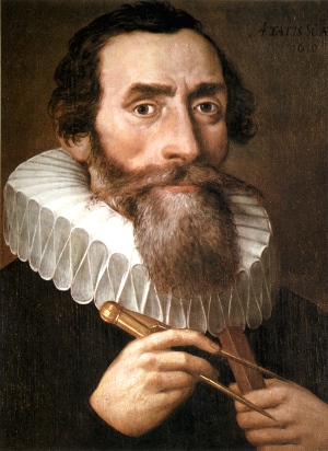
Johannes Kepler

The contraction mapping theorem says that if a function moves points closer together, then there must be some point the function doesn’t move. We’ll make this statement more precise and give a historically important application.

Definitions and theorem

A function f on a metric space X is a contraction if there exists a constant q with 0 ≤ q < 1 such that for any pair of points x and y in X,

d( f(x),  f(y) ) ≤ q d(xy)

where d is the metric on X.

A point x is a fixed point of a function f if f(x) = x.

Banach’s fixed point theorem, also known as the contraction mapping theorem, says that every contraction on a complete metric space has a fixed point. The proof is constructive: start with any point in the space and repeatedly apply the contraction. The sequence of iterates will converge to the fixed point.

Application: Kepler’s equation

Kepler’s equation in for an object in an elliptical orbit says

Me sin EE

where M is the mean anomalye is the eccentricity, and E is the eccentric anomaly. These “anomalies” are parameters that describe the location of an object in orbit. Kepler solved for E given M and e using the contraction mapping theorem, though he didn’t call it that.

Kepler speculated that it is not possible to solve for E in closed form—he was right—and used a couple iterations [1] of

f(E) = M + e sin E

to find an approximate fixed point. Since the mean anomaly is a good approximation for the eccentric anomaly, M makes a good starting point for the iteration. The iteration will converge from any starting point, as we will show below, but you’ll get a useful answer sooner starting from a good approximation.

Proof of convergence

Kepler came up with his idea for finding E around 1620, and Banach stated his fixed point theorem three centuries later. Kepler had the idea of Banach’s theorem, but he didn’t have a rigorous formulation of the theorem or a proof.

In modern terminology, the real line is a complete metric space and so we only need to prove that the function f above is a contraction. By the mean value theorem, it suffices to show that the absolute value of its derivative is less than 1. That is, we can use an upper bound on |‘| as the q in the definition of contraction.

Now

f ‘ (E) = e cos E

and so

|f ‘(E)| ≤ e

for all E. If our object is in an elliptical orbit, e < 1 and so we have a contraction.

Example

The following example comes from [2], though the author uses Newton’s method to solve Kepler’s equation. This is more efficient, but anachronistic.

Consider a satellite on a geocentric orbit with eccentricity e = 0.37255. Determine the true anomaly at three hours after perigee passage, and calculate the position of the satellite.

The author determines that M = 3.6029 and solves Kepler’s equation

Me sin EE

for E, which she then uses to solve for the true anomaly and position of the satellite.

The following Python code shows the results of the first 10 iterations of Kepler’s equation.

    from math import sin

    M = 3.6029
    e = 0.37255

    E = M
    for _ in range(10):
        E = M + e*sin(E)
        print(E)

This produces

    3.437070
    3.494414
    3.474166
    3.481271
    3.478772
    3.479650
    3.479341
    3.479450
    3.479412
    3.479425

and so it appears the iteration has converged to E = 3.4794 to four decimal places.

Note that this example has a fairly large eccentricity. Presumably Kepler would have been concerned with much smaller eccentricities. The eccentricity of Jupiter’s orbit, for example, is around 0.05. For such small values of e the iteration would converge more quickly.

Update: See this post for more efficient ways to solve Kepler’s equation.

Related posts

[1] Bertil Gustafsson saying in his book Scientific Computing: A Historical Perspective that Kepler only used two iterations. Since M gives a good starting approximation to E, two iterations would give a good answer. I imagine Kepler would have done more iterations if necessary but found empirically that two was enough. Incidentally, it appears Gustaffson has a sign error in his statement of Kepler’s equation.

[2] Euler Celestial Analysis by Dora Musielak.