Safe Harbor ain’t gonna cut it

There are two ways to deidentify data to satisfy HIPAA:

  • Safe Harbor, § 164.514(b)(2), and
  • Expert Determination, § 164.514(b)(1).

And for reasons explained here, you may need to be concerned with HIPAA even if you’re not a “covered entity” under the statute.

To comply with Safe Harbor, your data may not contain any of eighteen categories of information. Most of these are obvious: direct identifiers such as name, phone number, email address, etc. But some restrictions under Safe Harbor are less obvious and more difficult to comply with.

For example, under Safe Harbor you need to remove

All elements of dates (except year) for dates that are directly related to an individual, including birth date, admission date, discharge date, death date, and all ages over 89 and all elements of dates (including year) indicative of such age, except that such ages and elements may be aggregated into a single category of age 90 or older.

This would make it impossible, for example, to look at seasonal trends in medical procedures because you would only have data to the resolution of a year. But with a more sophisticated approach, e.g. differential privacy, it would be possible to answer such questions while providing better privacy for individuals. See how here.

If you need to comply with HIPAA, or analogous state laws such as TMPRA, and you can’t follow Safe Harbor, your alternative is expert determination. If you’d like to discuss expert determination, let’s talk.

Inverse congruence RNG

Linear congruence random number generators have the form

xn+1 = a xn + b mod p

Inverse congruence generators have the form

xn+1 = a xn−1 + b mod p

were x−1 means the modular inverse of x, i.e. the value y such that xy = 1 mod p. It is possible that x = 0 and so it doesn’t have an inverse. In that case the generator returns b.

Linear congruence generators are quite common. Inverse congruence generators are much less common.

Inverse congruence generators were first proposed by J. Eichenauer and J. Lehn in 1986. (The authors call them inversive congruential generators; I find “inverse congruence” easier to say than “inversive congruential.”)

An advantage of such generators is that they have none of the lattice structure that can be troublesome for linear congruence generators. This could be useful, for example, in high-dimensional Monte Carlo integration.

These generators are slow, especially in Python. They could be implemented more efficiently in C, and would be fast enough for applications like Monte Carlo integration where random number generation isn’t typically the bottleneck.

The parameters a, b, and p have to satisfy certain algebraic properties. The parameters I’ll use in the post were taken from [1]. With these parameters the generator has maximal period p.

The generator naturally returns integers between 0 and p. If that’s what you want, then the state and the random output are the same.

If you want to generate uniformly distributed real numbers, replace x above with the RNG state, and let x be the state divided by p. Since p has 63 bits and a floating point number has 53 significant bits, all the bits of the result should be good.

Here’s a Python implementation for uniform floating point values. We pass in x and the state each time to avoid global variables.

    from sympy import mod_inverse

    p = 2**63 - 25
    a = 5520335699031059059
    b = 2752743153957480735

    def icg(pair):
        x, state = pair
        if state == 0:
            return (b/p, b)
        else:
            state = (a*mod_inverse(state, p) + b)%p
        return (state/p, state)

If you’re running Python 3.8 or later, you can replace

    mod_inverse(state, p)

with

    pow(state, -1, p)

and not import sympy.

Here’s an example of calling icg to print 10 floating point values.

    x, state = 1, 1
    for _ in range(10):
        (x, state) = icg((x, state))
        print(x)

If we want to generate random bits rather than floating point numbers, we have to work a little harder. If we just take the top 32 bits, our results will be slightly biased since our output is uniformly distributed between 0 and p, not between 0 and a power of 2. This might not be a problem, depending on the application, since p is so near a power of 2.

To prevent this bias, I used a acceptance-rejection sampling method, trying again when the method generates a value above the largest multiple of 232 less than p. The code should nearly always accept.

    T = 2**32
    m = p - p%T

    def icg32(pair):
        x, state = pair
        if state == 0:
            return (b % T, b)
        state = (a*mod_inverse(state, p) + b)%p
        while state > m:  # rare
            state = (a*mod_inverse(state, p) + b)%p
        return (state % T, state)

You could replace the last line above with

    return state >> (63-32)

which should be more efficient.

The generator passes the four most commonly used test suites

  • DIEHARDER
  • NIST STS
  • PractRand
  • TestU01

whether you reduce the state mod 32 or take the top 32 bits of the state. I ran the “small crush” battery of the TestU01 test suite and all tests passed. I didn’t take the time to run the larger “crush” and “big crush” batteries because they require two and three orders of magnitude longer.

More on random number generation

[1] Jürgen Eichenauer-Herrmann. Inversive Congruential Pseudorandom Numbers: A Tutorial. International Statistical Review, Vol. 60, No. 2, pp. 167–176.

A better adaptive Runge-Kutta method

This is the third post in a series on Runge-Kutta methods. The first post in the series introduces Runge-Kutta methods and Butcher tableau. The next post looked at Fehlberg’s adaptive Runge-Kutta method, first published in 1969. This post looks at a similar method from Dormand and Prince in 1980.

Like Fehlberg’s method, the method of Dormand and Prince can be summarized in a big, intimidating tableau, which we will display below. However we will discuss three differences between the methods:

  • Order 4(5) vs 5(4)
  • Derivative reuse
  • Precision / computation ratio

Dormand Prince tableau

Here’s the Butcher tableau for the Dormand-Prince method in all it’s glory:

Dormand-Prince tableau

The only detail of the table that will be important below is that 7th and 8th rows are identical.

Order 4(5) vs order 5(4)

Fehlberg’s method, a.k.a. RKF45, computes each update to the solution using a 4th order Runge-Kutta method, and uses a 5th order Runge-Kutta method to estimate the error.

The method of Dormand and Prince also uses 4th and 5th order Runge-Kutta methods, but in the opposite way. The fifth order method is used to advance the solution, and the 4th order method is used for comparison to estimate error.

Derivative reuse

The work in solving

y' = f(t, y)

by a Runge-Kutta method is roughly proportional to the number of stages. Dormand-Prince is a 7-stage method while Fehlberg is a 6-stage method, so it would seem that the latter is more efficient. However, if you look back at the Dormand-Prince tableau, the last row above the horizontal line equals the first row below the line. That means that the last evaluation of f at one step can be reused at the first evaluation of f at the next step.

Precision per unit work

In their book Solving Differential Equations, vol. 1, Hairer et al compare several adaptive Runge-Kutta methods, including Fehlberg (RKF45) and Dormand-Prince, and conclude that the latter produces more precision per unit work.

We again see that the [Fehlberg] method underestimates the local error. Further, with the use of local extrapolation, the advantage of RKF4(5) melts away to a large extent. The best method of all these is without a doubt the coefficient set of Dormand and Prince.

More differential equation posts

How to estimate ODE solver error

This post brings together several themes I’ve been writing about lately: caching function evaluations, error estimation, and Runge-Kutta methods.

A few days ago I wrote about how Runge-Kutta methods can all be summarized by a set of numbers called the Butcher tableau. These methods solve

y' = f(t, y)

by evaluating f at some partial step, then evaluating f again at some new partial step and some linear combination of values from previous steps, etc. In the preface to J. C. Butcher’s book on differential equations, JM Sanz-Serna describes this structure as follows.

Runge-Kutta schemes … are highly nonlinear with a remarkable Matrioshka doll structure, where the vector field has to be evaluated an expression that involves the vector field evaluated at and expression that involves the vector field …

Once all the “Matrioshka dolls” are lined up, i.e. all the intermediate results have been calculated, the final estimate is a linear combination of these values.

Here’s the clever idea behind adaptive solvers: Create two Runge-Kutta methods of different orders that depend on the same intermediate results. Then both can be computed without new function evaluations, and the results compared. The difference between the results can be used as an estimate of the local error. Then you can adjust your step size accordingly and try again.

I’m going to present two adaptive Runge-Kutta schemes. I’ll go over Fehlberg’s method in this post and a variation in the next post that has some advantages over Fehlberg’s method.

Runge-Kutta-Felhberg (RKF45)

Fehlberg’s method, commonly known as RKF45, starts with a six-stage Runge Kutta method whose coefficients are given by the following tableau.


\begin{array} {c|ccccccc} 0\\ 1/4 & 1/4 \\ 3/8 & 3/32 & 9/32 \\ 12/13 & 1932/2197 & -7200/2197 & 7296/2197 \\ 1 & 439/216 & -8 & 3680/513 & -845/4104 \\ 1/2 & -8/27 & 2 & -3544/2565 & 1859/4104 & -11/40 \\ \hline y_1 & 25/216 & 0 & 1408/2565 & 2197/4104 & -1/5 & 0 & \\ \hline \hat{y} & 16/135 & 0 & 6656/12825 & 28561/56430 & -9/50 & 2/55 \end{array}

The meaning of the tableau is described here. (Imagine the effort it took Erwin Felhberg to derive this in 1969. Presumably he had little more than a desktop calculator to help. Maybe not even that.)

What’s important about the tableau for this post is that the coefficients above the horizontal line are used to create six numbers, the k‘s in the notation of the post referenced above. The k‘s are multiplied by the coefficients below the horizontal line to produce the solution of the differential equation at the next step. This is the “4” of RKF45.

RKF45 then applies another method which reuses all the k‘s in a different linear combination. This is summarized in the following variation of the Butcher tableau.

\begin{array} {c|ccccccc} 0\\ 1/4 & 1/4 \\ 3/8 & 3/32 & 9/32 \\ 12/13 & 1932/2197 & -7200/2197 & 7296/2197 \\ 1 & 439/216 & -8 & 3680/513 & -845/4104 \\ 1/2 & -8/27 & 2 & -3544/2565 & 1859/4104 & -11/40 \\ \hline y_1 & 25/216 & 0 & 1408/2565 & 2197/1404 & -1/5 & 0 & \\ \hline \hat{y} & 16/135 & 0 & 6656/12825 & 28561/56430 & -9/50 & 2/55 \end{array}

This is essentially two tableau combined into one. The first is as above. The second is like the one above but with a different bottom row. The bottom row gives the coefficients for a Runge-Kutta method corresponding to the “5” part of RKF45.

The 4 stands for 4th order, i.e. the local error for a step size h is O(h4). The 5 stands for 5th order, i.e. local error O(h5). RKF45 is two different methods, but they share so much computation that the second one almost comes for free; it does not require any new function evaluations, only taking a linear combination of six numbers.

However, RK45 is only “free” if you’ve gone to the effort of using a six-stage method. The amount of computation is roughly proportional to the number of stages, so we do about 50% more work to have RKF45 with an error estimate than doing the most common 4th order RK method. So if you knew exactly what step size to use, basic RK would be more efficient. But how could you know the optimal step size a priori?

By guiding us to choose the right step size, the extra work in RKF45 more than pays for itself. It could save a lot of computation that would come from using too small a step size, or prevent inaccurate results due to using too large a step size. Or maybe both: maybe a differential equation needs small steps at one period of time and can use larger steps at another period of time.

For more information on Felhberg’s method, see Solving Differential Equations by Hairer et al.

Related posts

Trapezoid rule and Romberg integration

This post will look at two numerical integration methods, the trapezoid rule and Romberg’s algorithm, and memoization. This post is a continuation of ideas from the recent posts on Lobatto integration and memoization.

Although the trapezoid rule is not typically very accurate, it can be in special instances, and Romberg combined it with extrapolation to create a very accurate method.

Trapezoid rule

The trapezoid is the simplest numerical integration method. The only thing that could be simpler is Riemann sums. By replacing rectangles of Riemann sums with trapezoids, you can make the approximation error an order of magnitude smaller.

The trapezoid rule is crude, and hardly recommended for practical use, with two exceptions. It can be remarkably efficient for periodic functions and for analytic functions that decay double exponentially. The trapezoid rule works so well in these cases that it’s common to transform a general function so that it has one of these forms so the trapezoid rule can be applied.

To be clear, the trapezoid rule for a given step size h may not be very accurate. But for periodic and double exponential functions the error decreases exponentially as h decreases.

Here’s an implementation of the trapezoid rule that follows the derivation directly.

    def trapezoid1(f, a, b, n):
        integral = 0
        h = (b-a)/n
        for i in range(n):
            integral += 0.5*h*(f(a + i*h) + f(a + (i+1)*h))
        return integral

This code approximates the integral of f(x) over [a, b] by adding up the areas of n trapezoids. Although we want to keep things simple, a slight change would make this code twice as efficient.

    def trapezoid2(f, a, b, n):
        integral = 0.5*( f(a) + f(b) )
        h = (b-a)/n
        for i in range(1, n):
            integral += f(a + i*h)
        return h*integral

Now we’re not evaluating f twice at every interior point.

Estimating error

Suppose you’ve used the trapezoid rule once, then you decide to use it again with half as large a step size in order to compare the results. If the results are the same within your tolerance, then presumably you have your result. Someone could create a function where this comparison would be misleading, where the two results agree but both are way off. But this is unlikely to happen in practice. As Einstein said, God is subtle but he is not malicious.

If you cut your step size h in half, you double your number of integration points. So if you evaluated your integrand at n points the first time, you’ll evaluate it at 2n points the second time. But half of these points are duplicates. It would be more efficient to save the function evaluations from the first integration and reuse them in the second integration, only evaluating your function at the n new integration points.

It would be most efficient to write your code to directly save previous results, but using memoization would be easier and still more efficient than redundantly evaluating your integrand. We’ll illustrate this with Python code.

Now let’s integrate exp(cos(x)) over [0, π] with 4 and then 8 steps.

    from numpy import exp, cos, pi

    print( trapezoid2(f, 0, pi, 4) )
    print( trapezoid2(f, 0, pi, 8) )

This prints

    3.97746388
    3.97746326

So this suggests we’ve already found our integral to six decimal places. Why so fast? Because we’re integrating a periodic function. If we repeat our experiment with exp(x) we see that we don’t even get one decimal place agreement. The code

    print( trapezoid2(exp, 0, pi, 4 ) )
    print( trapezoid2(exp, 0, pi, 8 ) )

prints

    23.26
    22.42

Eliminating redundancy

The function trapezoid2 eliminated some redundancy, but we still have redundant function evaluations when we call this function twice as we do above. When we call trapezoid2 with n = 4, we do 5 function evaluations. When we call it again with n = 8 we do 9 function evaluations, 4 of which we’ve done before.

As we did in the Lobatto quadrature example, we will have our integrand function sleep for 10 seconds to make the function calls obvious, and we will add memoization to have Python to cache function evaluations for us.

    from time import sleep, time
    from functools import lru_cache

    @lru_cache()
    def f(x):
        sleep(10)
        return exp(cos(x))

    t0 = time()
    trapezoid2(f, 0, pi, 4)
    t1 = time()
    print(t1 - t0)
    trapezoid2(f, 0, pi, 8)
    t2 = time()
    print(t2 - t1)

This shows that the first integration takes 50 seconds and the second requires 40 seconds. The first integration requires 5 function evaluations and the second requires 9, but the latter is faster because it only requires 4 new function evaluations.

Romberg integration

In the examples above, we doubled the number of integration intervals and compared results in order to estimate our numerical integration error. A natural next step would be to double the number of intervals again. Maybe by comparing three integrations we can see a pattern and project what the error would be if we did more integrations.

Werner Romberg took this a step further. Rather than doing a few integrations and eye-balling the results, he formalized the inference using Richardson extrapolation to project where the integrations are going. Specifically, his method applies the trapezoid rule at 2m points for increasing values of m. The method stops when either the maximum value of m has been reached or the difference between successive integral estimates is within tolerance. When Romberg’s method is appropriate, it converges very quickly and there is no need for m to be large.

To illustrate Romberg’s method, let’s go back to the example of integrating exp(x) over [0, π]. If we were to use the trapezoid rule repeatedly, we would get these results.

     Steps    Results
         1  37.920111
         2  26.516336
         4  23.267285
         8  22.424495
        16  22.211780
        32  22.158473

This doesn’t look promising. We don’t appear to have even the first decimal correct. But Romberg’s method applies Richardson extrapolation to the data above to produce a very accurate result.

    from scipy.integrate import romberg

    r = romberg(exp, 0, pi, divmax = 5) 
    print("exact:   ", exp(pi) - 1)
    print("romberg: ", r)

This produces

    exact:    22.1406926327792
    romberg:  22.1406926327867

showing that although none of the trapezoid rule estimates are good to more than 3 significant figures, the extrapolated estimate is good 12 figures, almost to 13 figures.

If you pass the argument show=True to romberg you can see the inner workings of the integration, including a report that the integrand was evaluated 33 times, i.e. 1 + 2m times when m is given by divmax.

It seems mysterious how Richardson extrapolation could take the integral estimates above, good to three figures, and produce an estimate good to twelve figures. But if we plot the error in each estimate on a log scale it becomes more apparent what’s going on.
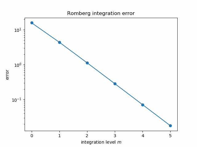
Plot of error in Romberg integration

The errors follow nearly a straight line, and so the extrapolated error is “nearly” negative infinity. That is, since the log errors nearly follow a straight line going down, polynomial extrapolation produces a value whose log error is very large and negative.

More on numerical integration

Python and the Tell-Tale Heart

I was browsing through SciPy documentation this evening and ran across a function in scipy.misc called electrocardiogram. What?!

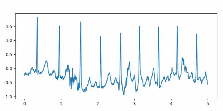
It’s an actual electrocardiogram, sampled at 360 Hz. Presumably it’s included as convenient example data. Here’s a plot of the first five seconds.

ECG plot

I wrote a little code using it to turn the ECG into an audio file.

from numpy import int16, iinfo
from scipy.io.wavfile import write
from scipy.misc import electrocardiogram

def to_integer(signal):
    # Take samples in [-1, 1] then scale to 16-bit integers
    m = iinfo(int16).max
    M = max(abs(signal))
    return int16(signal*m/M)

ecg = electrocardiogram()
write("heartbeat.wav", 360, to_integer(ecg))

I had to turn the volume way up to hear it, and that made me think of Edgar Allan Poe’s story The Tell-Tale Heart.

I may be doing something wrong. According to the documentation for the write function, I shouldn’t need to convert the signal to integers. I should just be able to leave the signal as floating point and normalize it to [−1, 1] by dividing by the largest absolute value in the signal. But when I do that, the output file will not play.

Related posts

Why HIPAA matters even if you’re not a “covered entity”

medical data

The HIPAA privacy rule only applies to “covered entities.” This generally means insurance plans, healthcare clearinghouses, and medical providers. If your company is using heath information but isn’t a covered entity per the HIPAA statute, there are a couple reasons you might still need to pay attention to HIPAA [1].

The first is that state laws may be broader than federal laws. For example, the Texas Medical Records Privacy Act extends the definition of covered entity to any business “assembling, collecting, analyzing, using, evaluating, storing, or transmitting protected health information.” So even if the US government does not consider your business to be a covered entity, the State of Texas might.

The second is that more recent privacy laws look to HIPAA. For example, it’s not clear yet what exactly California’s new privacy legislation CCPA will mean in practice, even though the law went into effect at the beginning of the year. Because HIPAA is well established and guidance documentation, companies needing to comply with CCPA are looking to HIPAA for precedent.

The connection between CCPA and HIPAA may be formalized into more than an analogy. There is a proposed amendment to CCPA that would introduce HIPAA-like expert determination for CCPA. (Update: This amendment, AB 713, was signed into law September 25, 2020.)

If you would like to discuss HIPAA deidentification or data privacy more generally, let’s talk.

More on HIPAA

[1] I advise lawyers on statistical matters, but I am not a lawyer. Nothing here should be considered legal advice. Ask your legal counsel if you need to comply with HIPAA, or with state laws analogous to HIPAA.


Scaling and memoization

The previous post explained that Lobatto’s integration method is more efficient than Gaussian quadrature when the end points of the interval need to be included as integration points. It mentioned that this is an advantage when you need to integrate over a sequence of contiguous intervals, say [1, 2] then [2, 3], because the function being integrated only needs to be evaluated at the common end points once.

This occurs in application, for example, when numerically solving differential equations. An integral might need to be evaluated at a sequence of contiguous intervals, one for each time step.

This post will illustrate the time savings from the combination of Lobatto integration and memoization. i.e. caching function evaluations. Some languages have a built-in feature for memoization. In other languages you may need to write your own memoization code.

Scaling

In order to integrate functions over intervals other than [−1, 1] we need a change of variables to rescale the domain. We’ll incorporate that in the code below.

Here is our code to integrate a function f over an interval [a, b].

    def lobatto(f, a, b):
        # Change integration interval to [-1, 1]
        c = (b-a)/2
        d = (b+a)/2
        # Multiply by c because c is the
        # Jacobian of the change of variables
        return c*integrate(lambda x: f(c*x + d),
            lobatto_points, lobatto_weights)

Reducing function evaluations

Next, we create a function to integrate which takes 10 second to evaluate. This is an artificial example, but the time required for numerical integration often is dominated by function evaluations. Here we choose an example that makes this obvious.

    from time import sleep, time

    def my_slow_function(x):
        sleep(10)
        return x**3 + x**2

The following code integrates my_slow_function over three contiguous intervals.

    t0 = time()
    lobatto(my_slow_function, 1, 2)
    lobatto(my_slow_function, 2, 3)
    lobatto(my_slow_function, 3, 4)
    t1 = time()
    print("Elapsed time: ", t1-t0)

This code takes 150 seconds because each integration requires five function evaluations at 10 seconds each.

However, by adding one line of code we can reduce the run time to 130 seconds. We add the decorator functools.lru_cache() to ask Python to cache evaluations of our integrand.

    @functools.lru_cache()
    def my_slow_function(x):
        sleep(10)
        return x**3 + x**2

Now the three integrations above take 130 seconds because my_slow_function is only evaluated at 2 and 3 one time each.

You could write your own code to cache function evaluations, and that might be worthwhile if efficiency is a priority, but it’s easy to let the language do it for you.

More on memoization

Lobatto integration

A basic idea in numerical integration is that if a method integrates polynomials exactly, it should do well on polynomial-like functions [1]. The higher the degree of polynomial it integrates exactly, the more accurate we expect it will be on functions that behave like polynomials.

The best known example of this is Gaussian quadrature. However, this post shows why for some applications you might want to use Lobatto quadrature instead. Lobatto quadrature is similar in spirit to Gaussian quadrature, but allocates points to solve a slightly different optimization problem.

Gaussian quadrature

If you need to integrate a function over an interval, it matters a great deal where you choose to evaluate the function. The optimal choice, in term of what polynomials you can integrate exactly, is to use Gaussian quadrature. By evaluating the integrand at n optimally chosen points you can integrate polynomials of degree 2− 1 or less exactly.

So if Gaussian integration is optimal, why would you want to do anything else? The Gaussian integration points are all interior to the interval of integration. In some applications, you have to evaluate your integrand at the end points, and so you want to optimize subject to a constraint: how can you best allocate your integration points subject to the constraint that two of your integration points are the two ends of the interval? The solution is Lobatto quadrature, also called Gauss-Lobatto quadrature.

Lobatto quadrature

By evaluating the integrand at n points, two of which are the end points, Lobatto’s method exactly integrates polynomials of degree 2n-3.

Suppose for whatever reason you already know the value of the integrand evaluated at the end points. You’ve got m more function evaluations to spend. If you use those m points for Gaussian quadrature, you can exactly integrate polynomials of degree

2− 1

or less. But if you use Lobatto quadrature, your m interior evaluations plus your two known values at the end points give you a total of m+2 function evaluations, and so can integrate polynomials of degree

2(m + 2) − 3 = 2m + 1

or less exactly, two degrees higher than if we had used Gaussian quadrature.

Next, suppose you only know the value of the function you’re integrating at one end point. Say you’ve already integrate f(x) over the interval [1, 2] using Lobatto quadrature, and now you want to integrate over [2, 3]. You already know the value f(2) from your previous integration.

Suppose you have m new function evaluations you can afford, and you don’t know f(3). If you use Lobatto quadrature, f(3) has to come out of your function evaluation budget, so you can afford m − 1 interior integration points. You then know the value of f(x) at m + 1 points: f(2) came for free, you evaluated f(x) at m − 1 interior points and at x = 3. This lets you exactly integrate polynomials of degree

2(m + 1) − 3 = 2m − 1

or less, the same as Gaussian quadrature. But if you then need to integrate over [3, 4], knowing f(3) gives you a head start on the next integration, and so on.

Weights and integration points

You can look up the weights and integration points for Gaussian quadrature and Lobatto quadrature in, for example, Abramowitz and Stegun.

There is a nice symmetry between the two integration methods: Gaussian quadrature uses integration points based on the zeros of Legendre polynomials, and weights that depend on the derivatives of these polynomials. Lobatto quadrature is the other way around: integration points are given by the zeros of derivatives of Legendre polynomials, and the weights involve the Legendre polynomials themselves.

Python example

Here we’ll implement the Gauss and Lobatto rules of order five. Most of the code is data on integration points and weights.

    gauss_points = [
        -0.906179845938664,
        -0.538469310105683,
        0.0,
        +0.538469310105683,
        +0.906179845938664
    ]
    
    gauss_weights = [
        0.23692688505618908,
        0.47862867049936647,
        0.5688888888888889,
        0.47862867049936647,    
        0.23692688505618908
    ]
    
    lobatto_points = [
        -1.0,
        -0.6546536707079771,
        0,
        +0.6546536707079771,
        +1.0
    ]
    
    lobatto_weights = [
        0.1,
        0.5444444444444444,
        0.7111111111111111,
        0.5444444444444444,
        0.1
    ]

The integration points and weights are symmetrical, so you could make the code more compact at the expense of making it a little more complicated. Putting the + in front of positive integration points is a little unconventional, but it emphasizes the symmetry by making the positive and negative weights align vertically.

Here’s our integration code:

    def integrate(f, xs, ws):
        return sum(f(xs[i])*ws[i] for i in range(5))

where we pass it the function to integrate and either Gauss data or Lobatto data.

The following verifies that with 5 integration points, Gauss should be able to exactly integrate a 9th order polynomial, and Lobatto should be able to integrate a 7th order polynomial.

    print( integrate(lambda x: x**9 + 1,
               gauss_points, gauss_weights) )

    print( integrate(lambda x: x**7 + 1,
               lobatto_points, lobatto_weights) )

Both print 2.0 as expected. The integral of an odd function over [−1, 1] is zero, and the integral of 1 over the same interval is 2.

Now let’s use both to integrate cosine over [−1, 1].

    print( integrate(cos, gauss_points, gauss_weights) )
    print( integrate(cos, lobatto_points, lobatto_weights) )

The exact integral is 2 sin(1). Here are the results.

    Exact:   1.682941969
    Gauss:   1.682941970
    Lobatto: 1.682942320

So Gauss is correct to 8, almost 9, decimal places, and Lobatto is correct to 5 decimal places.

Next, let’s hard code a 3rd order Gauss rule for comparison.

    def gauss3(f):
        k = 0.6**0.5
        s = f(-k)*5 + f(0)*8 + f(k)*5
        return s/9

We can verify that it integrates fifth order polynomials exactly:

    print(gauss3(lambda x: x**5 + 1))

and we can use it to integrate cosine:

    print(gauss3(cos))

This returns 1.68300, a little less accurate then the Lobatto rule above, illustrating that typically Lobatto will be more accurate than Gauss with the same number of function evaluations interior to the interval of integration.

More on numerical integration

[1] Polynomials can’t have horizontal asymptotes, for example, and so we should not be surprised that a method that integrates high order polynomials exactly could still do poorly on, say, a normal probability density.

Runge-Kutta methods and Butcher tableau

If you know one numerical method for solving ordinary differential equations, it’s probably Euler’s method. If you know two methods, the second is probably 4th order Runge-Kutta. It’s standard in classes on differential equations or numerical analysis to present Euler’s method as conceptually simple but inefficient introduction, then to present Runge-Kutta as a complicated but efficient alternative.

Runge-Kutta methods are a huge family of numerical methods with a wide variety of trade-offs: efficiency, accuracy, stability, etc. Euler’s method is a member of the Runge-Kutta family as are countless other variations. You could devote a career to studying Runge-Kutta methods, and some people have.

Beneath the complexity and variety, all Runge-Kutta methods have a common form that can be summarized by a matrix and two vectors. For explicit Runge-Kutta methods (ERK) the matrix is triangular, and for implicit Runge-Kutta methods (IRK) the matrix is full.

This summary of an RK method is known as a Butcher tableau, named after J. C. Butcher who classified RK methods.

“The” Runge-Kutta method

For example, let’s start with what students often take to be “the” Runge-Kutta method. This method approximates solutions to a differential equation of the form

y' = f(t, y)

by

y_{n+1} = y_n + \frac{h}{6}\left( k_{n1} + 2k_{n2} + 2k_{n3} + k_{n4}\right)

where

k_{n1} &=& f(t_n, y_n) \\ k_{n2} &=& f(t_n + 0.5h, y_n + 0.5hk_{n1}) \\ k_{n3} &=& f(t_n + 0.5h, y_n + 0.5hk_{n2}) \\ k_{n4} &=& f(t_n + h, y_n + hk_{n3}) \\

The Butcher tableau for this ERK method is

\begin{array} {c|cccc} 0\\ 1/2 & 1/2\\ 1/2 &0 &1/2 \\ 1& 0& 0& 1\\ \hline & 1/6 & 1/3 & 1/3 &1/6 \end{array}

The numbers along the left side are the coefficients of h in the first argument of f.

The numbers along the bottom are the coefficients of the ks in the expression for the value of y at the next step.

The numbers in the middle of the array are the coefficients of the ks in second argument  of f. Because this is an explicit method, each k only depends on the previous ks, and so the table of coefficients has a triangular form.

Runge-Kutta 3/8 rule

The method above is the most common 4th order ERK rule, there is another known as the 3/8 rule. It is a little less efficient and a little more accurate. A step of this rule is given by

y_{n+1} = y_n + \frac{h}{8}\left( k_{n1} + 3k_{n2} + 3k_{n3} + k_{n4}\right)

where

\begin{align*} k_{n1} &= f(t_n, y_n) \\ k_{n2} &= f(t_n + \frac{h}{3}, y_n + \frac{h}{3}k_{n1}) \\ k_{n3} &= f(t_n +\frac{2h}{3}, y_n -\frac{h}{3}k_{n1} + hk_{n2}) \\ k_{n4} &= f(t_n + h, y_n + h k_{n1} - h k_{n2} + hk_{n3}) \end{align*}

This method is summarized in the following Butcher tableau.

\begin{array} {c|cccc} 0\\ 1/3 & 1/3\\ 2/3 & -1/3 &1 \\ 1& 1& -1 & 1\\ \hline & 1/8 & 3/8 & 3/8 &1/8 \end{array}

This example makes it a little easier to see what’s going on since none of the coefficients in the triangular array are zero. Full detail is given in the section below.

General Explicit Runge-Kutta

The most general form of an ERK rule with s steps is

y_{n+1} = y_n + h \sum_{i-1}^s b_i k_{ni}

where

k_{ni} = f\left(x_n + c_i h, y_n + h \sum_{j=1}^{i-1} a_{ij} k_{nj}\right)

and the Butcher tableau is

\begin{array} {c|ccccc} 0\\ c_2 & a_{21}\\ c_3 & a_{31} & a_{32} \\ \vdots & \vdots & & \ddots \\ c_s& a_{s1}& a_{s2} & \cdots & a_{s,s-1}\\ \hline & b_1 & b_2 & \cdots & b_{s-1} & b_s \end{array}

General implicit Runge-Kutta

With explicit (ERK) methods, each k depends only on its predecessors. With implicit (IRK) methods each k potentially depends on each of the others. The matrix in the tableau is full, not triangular, and one must solve for the ks.

Now

k_{ni} = f\left(x_n + c_i h, y_n + h \sum_{j=1}^s a_{ij} k_{nj}\right)

with the sum going all the way up to s, and the Butcher tableau is

\begin{array} {c|ccccc} c_1 & a_{11} & a_{12} & \cdots & a_{1s} \\ c_2 & a_{21} & a_{22} & \cdots & a_{2s} \\ \vdots & \vdots & & \ddots & \vdots \\ c_s& a_{s1}& a_{s2} & \cdots & a_{s,s}\\ \hline & b_1 & b_2 & \cdots & b_{s} \end{array}

Implicit methods are more complicated to implement, and require more computation for a given step size. However, they are more stable for stiff differential equations and may allow larger steps. Implicit methods are less efficient when they’re not needed, and more efficient when they are needed.

Back to Euler’s method

I said at the top of the post that Euler’s method was a special case of Runge-Kutta. The Butcher tableau for the explicit (forward) Euler method is simply

 \begin{array} {c|c} 0 & 0\\ \hline & 1\end{array}

and the tableau for the implicit (backward) Euler method is just

\begin{array} {c|c} 1 & 1\\ \hline & 1\end{array}

In this post I say more about these two methods and compare their stability.

More on differential equations