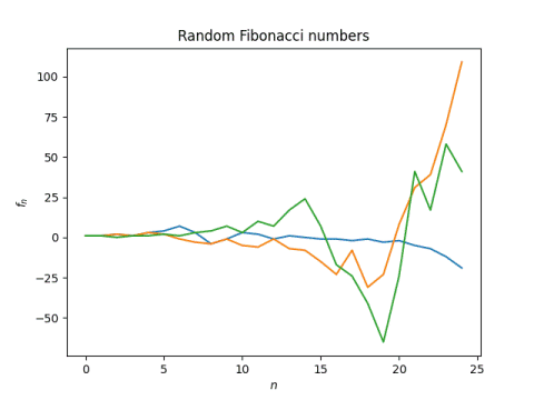
The previous post looked at random Fibonacci sequences. These are defined by

f₁ = f₂ = 1,

and

f_n = f_n−1 ± f_n−2

for n > 2, where the sign is chosen randomly to be +1 or −1.

Conjecture: Every integer can appear in a random Fibonacci sequence.

Here’s why I believe this might be true. The values in a random Fibonacci sequence of length n are bound between −F_n−3 and F_n.[1] This range grows like O(φⁿ) where φ is the golden ratio. But the number of ways to pick + and − signs in a random Fibonacci equals 2ⁿ.

By the pigeon hole principle, some choices of signs must lead to the same numbers: if you put 2ⁿ balls in φⁿ boxes, some boxes get more than one ball since φ < 2. That’s not quite rigorous since the range is  O(φⁿ) rather than exactly φⁿ, but that’s the idea. The graph included in the previous post shows multiple examples where different random Fibonacci sequences overlap.

Now the pigeon hole principle doesn’t show that the conjecture is true, but it suggests that there could be enough different sequences that it might be true. The fact that the ratio of balls to boxes grows exponentially doesn’t hurt either.

Empirically, it appears that as you look at longer and longer random Fibonacci sequences, gaps in the range are filled in.

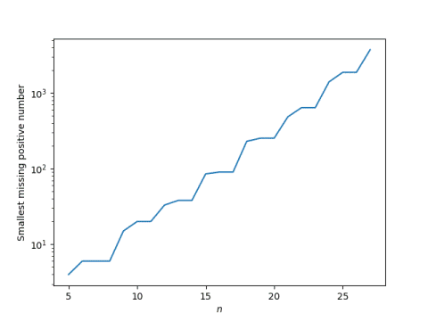
The following graphs consider all random Fibonacci sequences of length n, plotting the smallest positive integer and the largest negative integer not in the range. For the negative integers, we take the absolute value. Both plots are on a log scale.

First positive number missing:

Absolute value of first negative number missing:

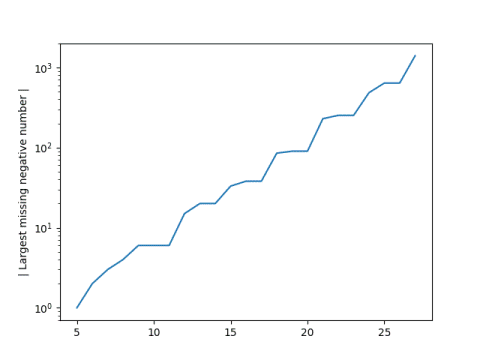
The span between the largest and smallest possible random Fibonacci sequence value is growing exponentially with n, and the range of consecutive numbers in the range is apparently also growing exponentially with n.

The following Python code was used to explore the gaps.

    import numpy as np
    from itertools import product

    def random_fib_range(N):
        r = set()
        x = np.ones(N, dtype=int)
        for signs in product((-1,1), repeat=(N-2)):
            for i in range(2, N):
                b = signs[i-2]
                x[i] = x[i-1] + b*x[i-2]
                r.add(x[i])
        return sorted(list(r)) 

    def stats(r):
        zero_location = r.index(0)

        # r is sorted, so these are the min and max values
        neg_gap = r[0]  // minimum
        pos_gap = r[-1] // maximum
     
        for i in range(zero_location-1, -1, -1):
            if r[i] != r[i+1] - 1:
                neg_gap = r[i+1] - 1
                break
        
        for i in range(zero_location+1, len(r)):
            if r[i] != r[i-1] + 1:
                pos_gap = r[i-1] + 1
                break
        
        return  (neg_gap, pos_gap)

    for N in range(5,25):
        r = random_fib_range(N)
        print(N, stats(r))

Proof

Update: Nathan Hannon gives a simple proof of the conjecture by induction in the comments.

You can create the series (1, 2) and (1, 3). Now assume you can create (1, n). Then you can create (1, n+2) via (1, n, n + 1, 1, n + 2). So you can create any positive even number starting from (1, 2) and any odd positive number from (1, 3).

You can do something analogous for negative numbers via (1, n, n − 1, −1, n − 2, n − 3, −1, 2 − n, 3 − n, 1, n − 2).

This proof can be used to create an upper bound on the time required to hit a given integer, and a lower bound on the probability of hitting a given integer during a random Fibonacci sequence.

Nathan’s construction requires more steps to produce new negative numbers, but that is consistent with the range of random Fibonacci sequences being wider on the positive side, [−F_n−3, F_n].

***

[1] To minimize the random Fibonacci sequence, you can chose the signs so that the values are 1, 1, 0, −1, −1, −2, −3, −5, … Note that absolute value of this sequence is the ordinary Fibonacci sequence with 3 extra terms spliced in. That’s why the lower bound is −F_n−3.

In a comment to my previous post on quatrefoils, Jan Van lint suggested a different equation for quatrefoils:

r = a + |cos(2θ)|

Here are some examples of how these curves look for varying values of a.

As a increases, the curves get rounder. We can quantify this by looking at the angle between the tangents on either side of the cusps. By symmetry, we can pick any one of the four cusps, so we’ll work with the one at θ = π/4 for convenience.

The slopes of the tangent lines are the left and right derivatives

Now the derivative of

a + |cos(2θ)|

with respect to θ at θ = π/4 is 2 from one size and -2 from the other.

Sine and cosine are equal at π/4, they cancel out in the ratio above and so the two derivatives, the slopes of the two tangent lines, are (2+a)/(2-a) and (2-a)/(2+a). The slopes are reciprocals of each other, which is what we’d expect since the quatrefoils are symmetric about the line θ = π/4.

The angles of the two tangent lines are the inverse tangents of the slopes, and so the angle between the two tangent lines is

Note that as a goes to zero, so does the angle between the tangent lines.

Here’s a plot of the angle as a function of a.

You could start with a desired angle and solve the equation above numerically for the value of a that gives the angle. From the graph above, it looks like if we wanted the curves to intersect at 90° we should pick a around 2. In fact, we should pick a exactly equal to 2. There the slopes are (2+2)/(2-2) = ∞ and (2-2)/(2+2) = 0, i.e. one tangent line is perfectly vertical and the other is perfectly horizontal.