Update on the Golay problem

I played around with what I’m calling the Golay problem over Christmas and wrote a blog post about it. I rewrote the post as I learned more about the problem due to experimentation and helpful feedback via comments and Twitter.

In short, the Golay problem is to classify the values of N and n such that

S(N, n) = \sum_{k=0}^n \binom{N}{k}

is a power of 2. It’s called the Golay problem because Marcel Golay discovered the solutions (23, 3) and (90, 2) in 1949. He used the former as the basis for the error correcting code that bears his name.

S(N, n) is a power of 2 if

  • n = 0 or n = N,
  • N is odd and n = (N-1)/2, or
  • n = 1 and N is one less than a power of two.

The only other solutions, as far as I know, are the two that Golay discovered.

I wrote a Python program to explore the problem, not intending to use it for large values of N. Then I became interested in searching further and it was clear that Python wouldn’t cut it. My son in law Aaron Smith offered to port the program to C using the GMP library, and the new code ran much faster.

The C code was about 40x faster for small values of N, and its speed advantage increases for larger values of N. I’ve currently verified that there are no more solutions up to N = 30,000.


Names and numbers for modal logic axioms

Stanislaw Ulam once said

Using a term like nonlinear science is like referring to the bulk of zoology as the study of non-elephant animals.

There is only one way to be linear, but there are many ways to not be linear.

A similar observation applies to non-classical logic. There are many ways to not be classical.

Modal logic axioms

Modal logic extends classical logic by adding modal operators □ and ◇. The interpretation of these operators depends on the application, but a common interpretation is “necessarily” and “possibly.”

There are a bewildering number of possible axioms to choose from in order to create a system of modal logic, and these often have cryptic names like “K”, “G”, and “5”. Seldom is any reason given for the names, and after digging into this a little, I think I know why: There isn’t much reason. Or rather, the reasons are historical rather than mnemonic.

For example, Axiom T is so named because Kurt Gödel published a paper that called some set of axioms “System T.” Of course that raises the question of why Gödel called his system “T.”

Axiom 5 gets its name from C. I. Lewis’ classification of logic systems. But Lewis’ numbering of systems S1 through S5 was essentially arbitrary, other than larger numbers corresponding to more axioms.

Unless you’re interested in the history for its own sake, it’s probably not worth questioning why rules are called what they are.

Lemmon numbering

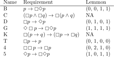
Although there’s not much logic behind the names of model logic axioms, there is a convenient way to catalog many of them. E. J. Lemmon [1] observed that many axioms for modal logic can be written in the form

\Diamond^i \Box^j p \to \Box^k \Diamond^\ell p

Here’s a list of some common modal logic axioms, along with their names and Lemmon numbers.

\begin{center} \begin{tabular}{lll} Name & Requirement & Lemmon \\ \hline B & \(p \to \boxempty \Diamond p\) & (0, 0, 1, 1) \\ C & \((\boxempty p \wedge \boxempty q) \to \boxempty (p \wedge q)\) & NA\\ D & \(\boxempty p \to \Diamond p\) & (0, 1, 0, 1)\\ G & \(\Diamond \boxempty p \to \boxempty \Diamond p\) & (1, 1, 1, 1)\\ K & \(\boxempty (p\to q) \to (\boxempty p \to \boxempty q)\) & NA \\ T & \(\boxempty p \to p\) & (0, 1, 0, 0) \\ 4 & \(\boxempty \! \boxempty p \to \boxempty p\) & (0, 2, 1, 0) \\ 5 & \(\Diamond p \to \boxempty \Diamond p\) & (1, 0, 1, 1) \\ \end{tabular} \end{center}

[1] E. J. Lemmon, An Introduction to Modal Logic, American Philosophical Quarterly, Monograph 11. Oxford, 1977.

When do two-body systems have stable Lagrange points?

The previous post looked at two of the five Lagrange points of the Sun-Earth system. These points, L1 and L2, are located on either side of Earth along a line between the Earth and the Sun. The third Lagrange point, L3, is located along that same line, but on the opposite side of the Sun.

L1, L2, and L3 are unstable, but stable enough on a short time scale to be useful places to position probes. Lagrange points are in the news this week because the James Webb Space Telescope (JWST), launched on Christmas Day, is headed toward L2 at the moment.

The remaining Lagrange points, L4 and L5, are stable. These points are essentially in Earth’s orbit around the Sun, 60° ahead and 60° behind Earth. To put it another way, they’re located where Earth will be in two months and where Earth was two months ago. The points L3, L4, and L5 form an equilateral triangle centered at the Sun.

Lagrange points more generally

Lagrange points are not unique to the Sun and Earth, but also holds for other systems as well. You have two bodies m1 and m2 , such as a star and a planet or a planet and a moon, and a third body, such as the JWST, with mass so much less than the other two that its mass is negligible compared to the other two bodies.

The L1, L2, and L3 points are always unstable, meaning that an object placed there will eventually leave, but the L4 and L5 points are stable, provided one of the bodies is sufficiently less massive than the other. This post will explore just how much less massive.

Mass ratio requirement

Michael Spivak [1] devotes a section of his physics book to the Trojan asteroids, asteroids that orbit the Sun at the L4 and L5 Lagrange points of a Sun-planet system. Most Trojan asteroids are part of the Sun-Jupiter system, but other planets have Trojan asteroids as well. The Earth has a couple Trojan asteroids of its own.

Spivak shows that in order for L4 and L5 to be stable, the masses of the two objects must satisfy

(m1m2) / (m1 + m2) > k

where m1 is the mass of the more massive body, m2 is the mass of the less massive body, and

k = √(23/27).

If we define r to be the ratio of the smaller mass to the larger mass,

r = m2 / m1,

then by dividing by m1 we see that equivalently we must have

(1 − r) / (1 + r) > k.

We run into the function (1 − z)/(1 + z) yet again. As we’ve pointed out before, this function is its own inverse, and so the solution for r is that

r < (1 − k) / (1 + k) = 0.04006…

In other words, the more massive body must be at least 25 times more massive than the smaller body.

The Sun is over 1000 times more massive than Jupiter, so Jupiter’s L4 and L5 Lagrange points with respect to the Sun are stable. The Earth is over 80 times more massive than the Moon, so the L4 and L5 points of the Earth-Moon system are stable as well.

Pluto has only 8 times the mass of its moon Charon, so the L4 and L5 points of the Pluto-Charon system would not be stable.

Related posts

[1] Michael Spivak: Physics for Mathematicians: Mechanics I. Addendum 10A.

Finding Lagrange points L1 and L2

The James Webb Space Telescope (JWST) is on its way to the Lagrange point L2 of the Sun-Earth system. Objects in this location will orbit the Sun at a fixed distance from Earth.

There are five Lagrange points, L1 through L5. The points L1, L2, and L3 are unstable, and points L4 and L5 are stable. Since L2 is unstable, it will have to adjust its orbit occasionally to stay at L2.

The Lagrange points L1 and L2 are nearly equally distant from Earth, with L1 between the Earth and Sun, and L2 on the opposite side of Earth from the Sun.

The equations for the distance r from L1 and L2 to Earth are very similar and can be combined into one equation:

\frac{M_1}{(R\pm r)^2} \pm \frac{M_2}{r^2}=\left(\frac{M_1}{M_1+M_2}R \pm r\right)\frac{M_1+M_2}{R^3}

The equation for L1 corresponds to taking ± as – and the equation for L2 corresponds to taking ± as +.

In the equation above, R is the distance between the Sun and Earth, and M1 and M2 are the mass of the Sun and Earth respectively. (This is not going to be too precise since the distance between the Sun and Earth is not constant. We’ll use the mean distance for R.)

For both L1 and L2 we have

r \approx R \sqrt[3]{\frac{M_2}{3M_1}}

Let’s use Newton’s method to solve for the distances to L1 and L2, and see how they compare to the approximation above.

    from scipy.optimize import newton
    
    M1 = 1.988e30 # kg
    M2 = 5.972e24 # kg
    R  = 1.471e8  # km

    approx = R*(M2/(3*M1))**(1/3)
    
    def f(r, sign):
        M = M1 + M2
        ret = M1/(R + sign*r)**2 + sign*M2/r**2
        ret -= (R*M1/M + sign*r)*M/R**3
        return ret
    
    L1 = newton(lambda r: f(r, -1), approx)
    L2 = newton(lambda r: f(r,  1), approx)
    
    print("L1       = ", L1)
    print("approx   = ", approx)
    print("L2       = ", L2)
    print("L1 error = ", (approx - L1)/L1)
    print("L2 error = ", (L2 - approx)/L2)    

This prints the following.

    
    L1       = 1467000
    approx   = 1472000
    L2       = 1477000
    L1 error = 0.3357%
    L2 error = 0.3312%

So L2 is slightly further away than L1. The approximate distance under-estimates L2 and over-estimates L1 both by about 0.33% [1].

L1 and L2 are about 4 times further away than the moon.

Related posts

[1] The approximation for r makes an excellent starting point. When I set the relative error target to 1e−5, Newton’s method converged in four iterations.

    full = newton(lambda r: f(r, 1), approx, tol=1e-5, full_output=True)
    print(full)

The exception case is normal

Sine and cosine have power series with simple coefficients, but tangent does not. Students are shocked when they see the power series for tangent because there is no simple expression for the power series coefficients unless you introduce Bernoulli numbers, and there’s no simple expression for Bernoulli numbers.

The perception is that sine and cosine are the usual case, and that tangent is exceptional. That’s because in homework problems and examples, sine and cosine are the usual case, and tangent is exceptional. But as is often the case, the pedagogically convenient case is the exception rather than the rule.

Of the six common trig functions—sine, cosine, tangent, secant, cosecant, cotangent—sine and cosine are the only ones with power series not involving Bernoulli numbers. The power series for most of the common trig functions require Bernoulli numbers.

Details

The functions cosecant and cotangent have a singularity at 0, so the power series for these functions at 0 are Laurant series rather than Taylor series, i.e. they involve negative as well as positive exponents. We will look at z csc(z) and z cot(z) because multiplying by z removes the singularity.

\begin{align*} \sin(z) &= \sum_{n=0}^\infty (-1)^n \frac{ z^{2n+1} }{ (2n+1)! } \\ \cos(z) &= \sum_{n=0}^\infty (-1)^n \frac{ z^{2n} }{ (2n)! } \\ \tan(z) &= \sum_{n=1}^\infty (-1)^{n-1} 4^n (4^n-1) B_{2n} \frac{ z^{2n-1} }{ (2n)! } \\ \text{sec}(z) &= \sum_{n=0}^\infty (-1)^n E_{2n} \frac{ z^{2n} }{ (2n)! } \\ z\text{cot}(z) &= \sum_{n=0}^\infty (-4)^n B_{2n} \frac{ z^{2n} }{ (2n)! } \\ z\text{csc}(z) &= \sum_{n=0}^\infty (-1)^{n-1} (2^{2n} - 2) B_{2n} \frac{ z^{2n} }{ (2n)! } \end{align*}

The series for secant doesn’t use Bernoulli numbers directly but rather Euler numbers. However, Bernoulli and Euler numbers are closely related.

\begin{align*} B_n &= \sum_{k=0}^{n-1} \binom{n-1}{k} \frac{n}{4^n - 2^n} E_k \\ E_n &= \sum_{k=1}^{n} \binom{n}{k-1} \frac{2^n - 4^n}{k} B_k \end{align*}

Related posts

Binomial sums and powers of 2

Marcel Golay noticed that

\binom{23}{0} + \binom{23}{1} + \binom{23}{2} + \binom{23}{3} = 2^{11}

and realized that this suggested it might be possible to create a perfect code of length 23. I wrote a Twitter thread on this that explains how this relates to coding theory (and to sporadic simple groups).

This made me wonder how common it is for cumulative sums of binomial coefficients to equal a power of 2.

Define

S(N, n) = \sum_{k=0}^n \binom{N}{k}

Golay’s observation could be expressed as saying

S(23, 3) = 211.

How often is S(N, n) a power of 2?

There are two easy cases. First,

S(N, 0) = 20

for all N because there’s only one way to not choose anything from a set of N items. Second,

S(N, N) = 2N

for all N. (Proof: apply the binomial theorem to (1 + 1)N.)

If N is odd, then we have

S(N, (N− 1)/2) = 2N−1

by symmetry of the binomial coefficients.

Also,

S(2p − 1, 1) = 2p

In summary, S(N, k) is a power of 2 if

  • k = 0 or k = N,
  • N is odd and k = (N − 1)/2, or
  • k = 1 and N is one less than a power of two.

Are there any more possibilities? Apparently not many.

The only exceptions I’ve found are (23, 3) and (90, 2). Those are the only possibilities for N < 10,000. (Update: Searched up to 30,000.)

Golay found both of these solutions and mentioned them in [1]. In Golay’s words, “A limited search has revealed two such cases.” He didn’t say how far he looked, and apparently he didn’t have a proof that these were the only exceptional solutions.

(This post has been edited several times since I first posted it, to reflect corrections and a better understanding of the problem.)

Related posts

[1] Golay, M. (1949). Notes on Digital Coding. Proc. IRE. 37: 657.

O Come, O Come, Emmanuel: condensing seven hymns into one

The Christmas hymn “O Come, O Come, Emmanuel” is a summary of the seven “O Antiphons,” sung on December 17 though 23, dating back to the 8th century [1]. The seven antiphons are

  1. O Sapientia
  2. O Adonai
  3. O Radix Jesse
  4. O Clavis David
  5. O Oriens
  6. O Rex Gentium
  7. O Emmanuel

The corresponding verses of “O Come, O Come, Emmanuel” begin with the lines below.

  1. O come, Thou Wisdom from on high
  2. O come, o come, thou lord of might
  3. O come, Thou Branch of Jesse’s stem
  4. O come, Thou Key of David, come
  5. O come, Thou Bright and Morning Star
  6. O come, Desire of nations, bind
  7. O come, O come, Emmanuel

[1] Mars Hill Audio Conversations O Come, O Come, Emmanuel: Malcolm Guite and J. A. C. Redford on the Advent O Antiphons

Error correcting code from octonions

Yesterday I wrote about how to multiply octets of real numbers, the octonions. Today I’ll show how to create an error correcting code from the octonions. In fact, we’ll create a perfect code in the sense explained below.

We’re going to make a code out of octonions over a binary field. That is, we’re going to work with octets of bits rather than octets of real numbers. Our code is going to produce 8-bit numbers which we can think of as octonions with components in each dimension equal to either 0 or 1, and we’ll carry out addition mod 2.

Basis of the code

The earlier post bootstrapped the multiplication facts for octonions from the equation

e1 e2 = e4

and two symmetry rules:

  1. You can shift the subscripts by a constant amount mod 7.
  2. You can permute each rule if you multiply by the sign of the permutation.

The first rule says we have the following equations:

e1 e2 = e4
e2 e3 = e5
e3 e4 = e6
e4 e5 = e7
e5 e6 = e1
e6 e7 = e2
e7 e1 = e3

Our code is going to be based on the complements of the triples in the multiplication rules above. For example, the first rule contains subscripts 1, 2, and 4, and so its complement contains subscripts 3, 5, 6, and 7. So we want the seven octonions

e3 + e5 + e6 + e7
e1 + e4 + e6 + e7
e1 + e2 + e5 + e7
e1 + e2 + e3 + e6
e2 + e3 + e4 + e7
e1 + e3 + e4 + e5
e2 + e4 + e5 + e6

and one more octonion, the sum of all the bases:

1 + e1 + e2 + e3 + e4 + e5 + e6 + e7

Our code will be spanned by these eight octonions. Written as 8-bit numbers, or code will be spanned by

00010111
01001011
01100101
01110010
00111001
01011100
00101110
11111111

Every pair of binary numbers above differs in four positions. We can verify this with the following Python code.

    from itertools import combinations, product

    def popcount(n):
        return bin(n).count('1')

    def hd(m, n): # Hamming distance
        return popcount(m ^ n)

    gen = [
        0b00010111,
        0b01001011,
        0b01100101,
        0b01110010,
        0b00111001,
        0b01011100,
        0b00101110,
        0b11111111,
    ]

    for pair in combinations(gen, 2):
        assert(hd(pair[0], pair[1]) == 4)

We didn’t need to import product for the code above, but we’ll need it below.

Note that the popcount of the XOR of two numbers counts how many places where their bit representations differ, i.e. it computes the Hamming distance between the two bit vectors.

Hamming code

The fact that the octets above spread out well, each being a Hamming distance of 4 from all the rest, suggests they could be useful in coding, and in fact the vectors above span the Hamming code (8, 4, 4).

These octets from the previous section will be the basis of our code, “basis” in the colloquial sense of a starting point. They span our set of code words, but they’re not a basis in the linear algebra sense because they are not linearly independent. The following code shows that the octets span a 4 dimensional space, i.e. you can make 24 different bit patterns by XORing together combinations of these octets.

    codewords = set()
    n = 4
    for b in combinations(gen, n):
        for coeff in product(range(2), repeat=n):
            s = 0
            for i in range(n):
                s ^= coeff[i]*b[i]
            codewords.add(s)

    assert(len(codewords) == 16)

The code tells that our octets have a span of size 16, i.e. 4 dimensions over a 2-bit field.

(Normally this would be presented by doing linear algebra, but I’m doing it by brute force just for variety. I assume readers who are more comfortable with code than math will appreciate this.)

Perfect codes

The Hamming (8, 4, 4) code is “perfect” in the sense that its packing radius equals its covering radius.

The packing diameter is the minimum distance between code words, and the packing radius is half the packing diameter.

The following code shows this is 2.

    packing_radius = min(
        hd(p[0], p[1]) for p in combinations(codewords, 2))/2
    print(packing_radius)

Since the packing diameter is 4, we can detect if up to 3 bits are corrupted: no bit pattern that differs from a code word in three positions is a code word.

The covering radius is the maximum distance from any vector to a code word. The following Python snippet shows that no 8-bit vector is a Hamming distance of more than 2 from a code word.

    def dist_to_codeword(n):
        return min(hd(n, c) for c in codewords)

    covering_radius = max(dist_to_codeword(n) for n in range(256))
    print(covering_radius)

More coding theory posts

Conjugate theorem for octonions

Yesterday I wrote about the fact that quaternions, unlike complex numbers, can form conjugates via a series of multiplications and additions. This post will show that you can do something similar with octonions.

If x is an octonion

x = r0 e0 + r1 e1 + … + r7 e7

where all the r‘s are real numbers. The conjugate flips the signs of all the components except the real component:

x* = r0 e0r1 e1 − … − r7 e7

The conjugate theorem is

x* = − (x + (e1 x) e1 + … (e7 x) e7) / 6

which is analogous to the theorem

q* = − (q + iqi + jqj + kqk) /2

for quaternions.

The internal parentheses are necessary because multiplication in octonions is not associative:

xyz

is ambiguous because it could mean

(xy)z

or

x(yz)

and the two are not necessarily equal.

The proof is also analogous to the proof given in the earlier post for quaternions. First work out what the effect is of multiplying on the left and right by one of the imaginary units, then add everything up. You’ll find that the real component is multiplied by -6 and the rest of the components are multiplied by 6.