A priori overfitting

The term overfitting usually describes fitting too complex a model to available data. But it is possible to overfit a model before there are any data.

An experimental design, such as a clinical trial, proposes some model to describe the data that will be collected. For simple, well-known models the behavior of the design may be known analytically. For more complex or novel methods, the behavior is evaluated via simulation.

If an experimental design makes strong assumptions about data, and is then simulated with scenarios that follow those assumptions, the design should work well. So designs must be evaluated using scenarios that do not exactly follow the model assumptions. Here lies a dilemma: how far should scenarios deviate from model assumptions? If they do not deviate at all, you don’t have a fair evaluation. But deviating too far is unreasonable as well: no method can be expected to work well when it’s assumptions are flagrantly violated.

With complex designs, it may not be clear to what extent scenarios deviate from modeling assumptions. The method may be robust to some kinds of deviations but not to others. Simulation scenarios for complex designs are samples from a high dimensional space, and it is impossible to adequately explore a high dimensional space with a small number of points. Even if these scenarios were chosen at random—which would be an improvement over manually selecting scenarios that present a method in the best light—how do you specify a probability distribution on the scenarios? You’re back to a variation on the previous problem.

Once you have the data in hand, you can try a complex model and see how well it fits. But with experimental design, the model is determined before there are any data, and thus there is no possibility of rejecting the model for being a poor fit. You might decide after its too late, after the data have been collected, that the model was a poor fit. However, retrospective model criticism is complicated for adaptive experimental designs because the model influenced which data were collected.

This is especially a problem for one-of-a-kind experimental designs. When evaluating experimental designs — not the data in the experiment but the experimental design itself—each experiment is one data point. With only one data point, it’s hard to criticize a design. This means we must rely on simulation, where it is possible to obtain many data points. However, this brings us back to the arbitrary choice of simulation scenarios. In this case there are no empirical data to test the model assumptions.

Related posts

Probability of long runs

Suppose you’ve written a program that randomly assigns test subjects to one of two treatments, A or B, with equal probability. The researcher using your program calls you to tell you that your software is broken because it has assigned treatment A to seven subjects in a row.

You might argue that the probability of seven A’s in a row is (1/2)7 or about 0.008. Not impossible, but pretty small. Maybe the software is broken.

But this line of reasoning grossly underestimates the probability of a run of 7 identical assignments. If someone asked the probability that the next 7 assignments would all be A’s, then (1/2)7 would be the right answer. But that’s not the same as asking whether an experiment is likely to see a run of length 7 because the run could start any time, not just on the next assignment. Also, the phone didn’t ring out of the blue: it rang precisely because there had just been a run.

Suppose you have a coin that has probability of heads p and you flip this coin n times. A rule of thumb says that the expected length of the longest run of heads is about

-frac{log n(1-p)}{log p}

provided that n(1-p) is much larger than 1.

So in a trial of n = 200 subjects with p = 0.5, you’d expect the longest run of heads to be about seven in a row. When p is larger than 0.5, the longest expected run will be longer. For example, if p = 0.6, you’d expect a run of about 9.

The standard deviation of the longest run length is roughly 1/log(1/p), independent of n. For coin flips with equal probability of heads or tails, this says an approximate 95% confidence interval would be about 3 either side of the point estimate. So for 200 tosses of a fair coin, you’d expect the longest run of heads to be about 7 ± 3, or between 4 and 10.

The following Python code gives an estimate of the probability that the longest run is between a and b inclusive, based on an extreme value distribution.

def prob(a, b, n, p):
    r = -log(n*(1-p))/log(p)
    cdf = lambda x: exp(- p**x )
    return cdf(b + 1 - r) - cdf(a - r)

What if you were interested in the longest run of head or tails? With a fair coin, this just adds 1 to the estimates above. To see this, consider a success to be when consecutive coins turn up the same way. This new sequence has the same expected run lengths, but a run of length m in this sequence corresponds to a run of length m + 1 in the original sequence.

For more details, see “The Surprising Predictability of Long Runs” by Mark F. Schilling, Mathematics Magazine 85 (2012), number 2, pages 141–149.

RelatedNeed help with randomization?

Volatility in adaptive randomization

Randomized clinical trials essentially flip a coin to assign patients to treatment arms. Outcome-adaptive randomization “bends” the coin to favor what appears to be the better treatment at the time each randomized assignment is made. The method aims to treat more patients in the trial effectively, and on average it succeeds.

However, looking only at the average number of patients assigned to each treatment arm conceals the fact that the number of patients assigned to each arm can be surprisingly variable compared to equal randomization.

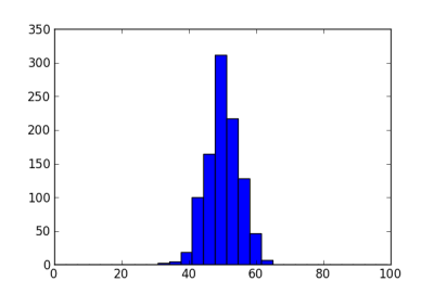
Suppose we have 100 patients to enroll in a clinical trial. If we assign each patient to a treatment arm with probability 1/2, there will be about 50 patients on each treatment. The following histogram shows the number of patients assigned to the first treatment arm in 1000 simulations. The standard deviation is about 5.

Next we let the randomization probability vary. Suppose the true probability of response is 50% on one arm and 70% on the other. We model the probability of response on each arm as a beta distribution, starting from a uniform prior. We randomize to an arm with probability equal to the posterior probability that that arm has higher response. The histogram below shows the number of patients assigned to the better treatment in 1000 simulations.

The standard deviation in the number of patients is now about 17. Note that while most trials assign 50 or more patients to the better treatment, some trials in this simulation put less than 20 patients on this treatment. Not only will these trials treat patients less effectively, they will also have low statistical power (as will the trials that put nearly all the patients on the better arm).

The reason for this volatility is that the method can easily be mislead by early outcomes. With one or two early failures on an arm, the method could assign more patients to the other arm and not give the first arm a chance to redeem itself.

Because of this dynamic, various methods have been proposed to add “ballast” to adaptive randomization. See a comparison of three such methods here. These methods reduce the volatility in adaptive randomization, but do not eliminate it. For example, the following histogram shows the effect of adding a burn-in period to the example above, randomizing the first 20 patients equally.

The standard deviation is now 13.8, less than without the burn-in period, but still large compared to a standard deviation of 5 for equal randomization.

Another approach is to transform the randomization probability. If we use an exponential tuning parameter of 0.5, the sample standard deviation of the number of patients on the better arm is essentially the same, 13.4. If we combine a burn-in period of 20 and an exponential parameter of 0.5, the sample standard deviation is 11.7, still more than twice that of equal randomization.

Related

Personalized medicine

When I hear someone say “personalized medicine” I want to ask “as opposed to what?”

All medicine is personalized. If you are in an emergency room with a broken leg and the person next to you is lapsing into a diabetic coma, the two of you will be treated differently.

The aim of personalized medicine is to increase the degree of personalization, not to introduce personalization. In particular, there is the popular notion that it will become routine to sequence your DNA any time you receive medical attention, and that this sequence data will enable treatment uniquely customized for you. All we have to do is collect a lot of data and let computers sift through it. There are numerous reasons why this is incredibly naive. Here are three to start with.

  • Maybe the information relevant to treating your malady is in how DNA is expressed, not in the DNA per se, in which case a sequence of your genome would be useless. Or maybe the most important information is not genetic at all. The data may not contain the answer.
  • Maybe the information a doctor needs is not in one gene but in the interaction of 50 genes or 100 genes. Unless a small number of genes are involved, there is no way to explore the combinations by brute force. For example, the number of ways to select 5 genes out of 20,000 is 26,653,335,666,500,004,000. The number of ways to select 32 genes is over a googol, and there isn’t a googol of anything in the universe. Moore’s law will not get us around this impasse.
  • Most clinical trials use no biomarker information at all. It is exceptional to incorporate information from one biomarker. Investigating a handful of biomarkers in a single trial is statistically dubious. Blindly exploring tens of thousands of biomarkers is out of the question, at least with current approaches.

Genetic technology has the potential to incrementally increase the degree of personalization in medicine. But these discoveries will require new insight, and not simply more data and more computing power.

Related posts

How long will there be computer science departments?

When universities began to form computer science departments, there was some discussion over how long computer science departments would exist. Some thought that after a few years, computer science departments would have served their purpose and computer science would be absorbed into other departments that applied it.

It looks like computer science departments are here to stay, but that doesn’t mean that there are not territorial disputes. If other departments are not satisfied with the education their students are getting from the computer science department, they will start teaching their own computer science classes. This is happening now, to different extents in different places.

Some institutions have departments of bioinformatics or biomathematics. Will they always? Or will “bioinformatics” and “biomathematics” simply be “biology” in a few years?

Statisticians sometimes have their own departments, sometimes reside in mathematics departments, and sometimes are scattered to the four winds with de facto statisticians working in departments of education, political science, etc. It would be interesting to see which of these three options grows in the wake of “big data.” A fourth possibility is the formation of “data science” departments, essentially statistics departments with more respect for machine learning and with better marketing.

No doubt computer science, bioinformatics, and statistics will be hot areas for years to come, but the scope of academic departments by these names will change. At different institutions they may grow, shrink, or even disappear.

Academic departments argue that because their subject is important, their department is important. And any cut to their departmental budget is framed as a cut to the budget for their subject. But neither of these is necessarily true. Matt Briggs wrote about this yesterday in regard to philosophy. He argues that philosophy is important but that philosophy departments are not. He quotes Peter Kreeft:

Philosophy was not a “department” to its founders. They would have regarded the expression “philosophy department” as absurd as “love department.”

Love is important, but it doesn’t need to be a department. In fact, it’s so important that the idea of quarantining it to a department is absurd.

Computer science and statistics departments may shrink as their subjects diffuse throughout the academy. Their departments may not go away, but they may become more theoretical and more specialized. Already most statistics education takes place outside of statistics departments, and the same may be true of computer science soon if it isn’t already.

How do you justify that distribution?

Someone asked me yesterday how people justify probability distribution assumptions. Sometimes the most mystifying assumption is the first one: “Assume X is normally distributed …” Here are a few answers.

  1. Sometimes distribution assumptions are not justified.
  2. Sometimes distributions can be derived from fundamental principles. For example, there are axioms that uniquely specify a Poisson distribution.
  3. Sometimes distributions are justified on theoretical grounds. For example, large samples and the central limit theorem together may justify assuming that something is normally distributed.
  4. Often the choice of distribution is somewhat arbitrary, chosen by intuition or for convenience, and then empirically shown to work well enough.
  5. Sometimes a distribution can be a bad fit and still work well, depending on what you’re asking of it.

The last point is particularly interesting. It’s not hard to imagine that a poor fit would produce poor results. It’s surprising when a poor fit produces good results. Here’s an example of the latter.

Suppose you are testing a new drug and hoping that it improves how long patients live. You want to stop the clinical trial early if it looks like patients are living no longer than they would have on standard treatment. There is a Bayesian method for monitoring such experiments that assumes survival times have an exponential distribution. But survival times are not exponentially distributed, not even close.

The method works well because of the question being asked. The method is not being asked to accurately model the distribution of survival times for patients in the trial. It is only being asked to determine whether a trial should continue or stop, and it does a good job of doing so. Simulations show that the method makes the right decision with high probability, even when the actual survival times are not exponentially distributed.

More probability posts

Small data

Big data is getting a lot of buzz lately, but small data is interesting too. In some ways it’s more interesting. Because of limit theorems, a lot of things become dull in the large that are more interesting in the small.

When working with small data sets you have to accept that you will very often draw the wrong conclusion. You just can’t have high confidence in inference drawn from a small amount of data, unless you can do magic. But you do the best you can with what you have. You have to be content with the accuracy of your method relative to the amount of data available.

For example, a clinical trial may try to find the optimal dose of some new drug by giving the drug to only 30 patients. When you have five doses to test and only 30 patients, you’re just not going to find the right dose very often. You might want to assign 6 patients to each dose, but you can’t count on that. For safety reasons, you have to start at the lowest dose and work your way up cautiously, and that usually results in uneven allocation to doses, and thus less statistical power. And you might not treat all 30 patients. You might decide—possibly incorrectly—to stop the trial early because it appears that all doses are too toxic or ineffective. (This gives a glimpse of why testing drugs on people is a harder statistical problem than testing fertilizers on crops.)

Maybe your method finds the right answer 60% of the time, hardly a satisfying performance. But if alternative methods find the right answer 50% of the time under the same circumstances, your 60% looks great by comparison.

Related post: The law of medium numbers

Works well versus well understood

While I was looking up the Tukey quote in my earlier post, I ran another of his quotes:

The test of a good procedure is how well it works, not how well it is understood.

At some level, it’s hard to argue against this. Statistical procedures operate on empirical data, so it makes sense that the procedures themselves be evaluated empirically.

But I question whether we really know that a statistical procedure works well if it isn’t well understood. Specifically, I’m skeptical of complex statistical methods whose only credentials are a handful of simulations. “We don’t have any theoretical results, buy hey, it works well in practice. Just look at the simulations.”

Every method works well on the scenarios its author publishes, almost by definition. If the method didn’t handle a scenario well, the author would publish a different scenario. Even if the author didn’t select the most flattering scenarios, he or she may simply not have considered unflattering scenarios. The latter is particularly understandable, almost inevitable.

Simulation results would have more credibility if an adversary rather than an advocate chose the scenarios. Even so, an adversary and an advocate may share the same blind spots and not explore certain situations. Unless there’s a way to argue that a set of scenarios adequately samples the space of possible inputs, it’s hard to have a great deal of confidence in a method based on simulation results alone.

Related posts

Why drugs often list headache as a side-effect

In an interview on Biotech Nation, Gary Cupit made an offhand remark about why so many drugs list headache as a possible side-effect: clinical trial participants are often asked to abstain from coffee during the trial. That also explains why those who receive placebo often complain of headache as well.

Cupit’s company Somnus Therapeutics makes a sleep medication for people who have no trouble going to sleep but do have trouble staying asleep. The medication has a timed-release so that it is active only in the middle of the night when needed. One of the criteria by which the drug is evaluated is whether there is a lingering effect the next morning. Obviously researchers would like to eliminate coffee consumption as a confounding variable. But this contributes to the litany of side-effects that announcers must mumble in television commercials.

Related: Adaptive clinical trial design