Mystery curve

Posted on 3 June 2015 by John

This afternoon I got a review copy of the book Creating Symmetry: The Artful Mathematics of Wallpaper Patterns. Here’s a striking curves from near the beginning of the book, one that the author calls the “mystery curve.”

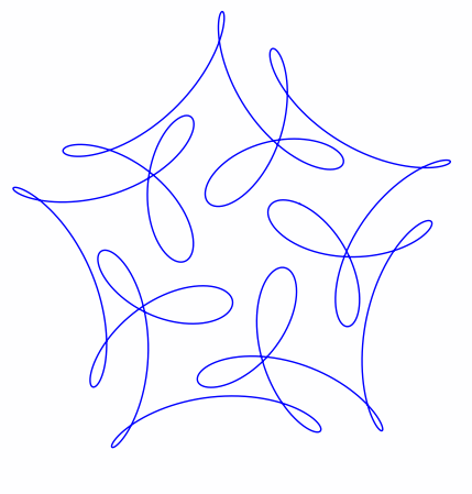
The curve is the plot of exp(it) − exp(6it)/2 + i exp(−14it)/3 with t running from 0 to 2π.

Here’s Python code to draw the curve.

    import matplotlib.pyplot as plt
    from numpy import pi, exp, real, imag, linspace

    def f(t):
        return exp(1j*t) - exp(6j*t)/2 + 1j*exp(-14j*t)/3

    t = linspace(0, 2*pi, 1000)

    plt.plot(real(f(t)), imag(f(t)))

    # These two lines make the aspect ratio square
    fig = plt.gcf()
    fig.gca().set_aspect('equal')

    plt.show()

Maybe there’s a more direct way to plot curves in the complex plane rather than taking real and imaginary parts.

Updated code for the aspect ratio per Janne’s suggestion in the comments.

Rotating PDF pages with Python

Posted on 1 May 2015 by John

Yesterday I got a review copy of Automate the Boring Stuff with Python. It explains, among other things, how to manipulate PDFs from Python. This morning I needed to rotate some pages in a PDF, so I decided to try out the method in the book.

The sample code uses PyPDF2. I’m using Conda for my Python environment, and PyPDF2 isn’t directly available for Conda. I searched Binstar with

binstar search -t conda pypdf2

The first hit was from JimInCO, so I installed PyPDF2 with

conda install -c https://conda.binstar.org/JimInCO pypdf2

I scanned a few pages from a book to PDF, turning the book around every other page, so half the pages in the PDF were upside down. I needed a script to rotate the even numbered pages. The script counts pages from 0, so it rotates the odd numbered pages from its perspective.

    import PyPDF2

    pdf_in = open('original.pdf', 'rb')
    pdf_reader = PyPDF2.PdfFileReader(pdf_in)
    pdf_writer = PyPDF2.PdfFileWriter()

    for pagenum in range(pdf_reader.numPages):
        page = pdf_reader.getPage(pagenum)
        if pagenum % 2:
            page.rotateClockwise(180)
        pdf_writer.addPage(page)

    pdf_out = open('rotated.pdf', 'wb')
    pdf_writer.write(pdf_out)
    pdf_out.close()
    pdf_in.close()

It worked as advertised on the first try.

Random walks and the arcsine law

Posted on 17 February 2015 by John

Suppose you stand at 0 and flip a fair coin. If the coin comes up heads, you take a step to the right. Otherwise you take a step to the left. How much of the time will you spend to the right of where you started?

As the number of steps N goes to infinity, the probability that the proportion of your time in positive territory is less than x approaches 2 arcsin(√x)/π. The arcsine term gives this rule its name, the arcsine law.

Here’s a little Python script to illustrate the arcsine law.

import random
from numpy import arcsin, pi, sqrt

def step():
    u = random.random()
    return 1 if u < 0.5 else -1

M = 1000 # outer loop
N = 1000 # inner loop

x = 0.3 # Use any 0 < x < 1 you'd like. 
outer_count = 0 
for _ in range(M): 
    n = 0 
    position= 0 
    inner_count = 0 
    for __ in range(N): 
        position += step() 
    if position > 0:
        inner_count += 1
    if inner_count/N < x:
        outer_count += 1

print (outer_count/M)
print (2*arcsin(sqrt(x))/pi)

Playing with continued fractions and Khinchin’s constant

Posted on 15 February 2015 by John

Take a real number x and expand it as a continued fraction. Compute the geometric mean of the first n coefficients.

Aleksandr Khinchin proved that for almost all real numbers x, as n → ∞ the geometric means converge. Not only that, they converge to the same constant, known as Khinchin’s constant, 2.685452001…. (“Almost all” here mean in the sense of measure theory: the set of real numbers that are exceptions to Khinchin’s theorem has measure zero.)

To get an idea how fast this convergence is, let’s start by looking at the continued fraction expansion of π. In Sage, we can type

continued_fraction(RealField(100)(pi))

to get the continued fraction coefficient

[3, 7, 15, 1, 292, 1, 1, 1, 2, 1, 3, 1, 14, 2, 1, 1, 2, 2, 2, 2, 1, 84, 2, 1, 1, 15, 3]

for π to 100 decimal places. The geometric mean of these coefficients is 2.84777288486, which only matches Khinchin’s constant to 1 significant figure.

Let’s try choosing random numbers and working with more decimal places.

There may be a more direct way to find geometric means in Sage, but here’s a function I wrote. It leaves off any leading zeros that would cause the geometric mean to be zero.

from numpy import exp, mean, log
def geometric_mean(x):
    return exp( mean([log(k) for k in x if k > 0]) )

Now let’s find 10 random numbers to 1,000 decimal places.

for _ in range(10):
    r = RealField(1000).random_element(0,1)
    print(geometric_mean(continued_fraction(r)))

This produced

2.66169890535
2.62280675227
2.61146463641
2.58515620064
2.58396664032
2.78152297661
2.55950338205
2.86878898900
2.70852612496
2.52689450535

Three of these agree with Khinchin’s constant to two significant figures but the rest agree only to one. Apparently the convergence is very slow.

If we go back to π, this time looking out 10,000 decimal places, we get a little closer:

print(geometric_mean(continued_fraction(RealField(10000)(pi))))

produces 2.67104567579, which differs from Khinchin’s constant by about 0.5%.

Python resources

Posted on 31 December 2014 by John

Each Wednesday I post a list of some of the resources on this site. This week: Python notes.

See also blog posts tagged Python, SciPy, and SymPy.

Last week: Special functions

Next week: Probability resources

Ellipsoid surface area

Posted on 6 July 2014 by John

How much difference does the earth’s equatorial bulge make in its surface area?

To first approximation, the earth is a sphere. The next step in sophistication is to model the earth as an ellipsoid.

The surface area of an ellipsoid with semi-axes a ≥ b ≥ c is

$A = 2\pi \left( c^2 + \frac{ab}{\sin\phi} \left( E(\phi, k) \sin^2\phi + F(\phi, k) \cos^2 \phi\right)\right)$

where

$\cos \phi = \frac{c}{a}$

and

$m = k^2 = \frac{a^2(b^2 - c^2)}{b^2(a^2 - c^2)}$

The functions E and F are incomplete elliptic integrals

$F(\phi, k) = \int_0^\phi \frac{d\theta}{\sqrt{1 - k^2 \sin^2\theta}}$

and

$E(\phi, k) = \int_0^\phi \sqrt{1 - k^2 \sin^2\theta}\,d\theta$

implemented in SciPy as ellipeinc and ellipkinc. Note that the SciPy functions take m as their second argument rather its square root k.

For the earth, a = b and so m = 1.

The following Python code computes the ratio of earth’s surface area as an ellipsoid to its area as a sphere.

from numpy import pi, sin, cos, arccos
from scipy.special import ellipkinc, ellipeinc

# values in meters based on GRS 80
# https://en.wikipedia.org/wiki/GRS_80
equatorial_radius = 6378137
polar_radius = 6356752.314140347

a = b = equatorial_radius
c = polar_radius

phi = arccos(c/a)
# in general, m = (a**2 * (b**2 - c**2)) / (b**2 * (a**2 - c**2))
m = 1

temp = ellipeinc(phi, m)*sin(phi)**2 + ellipkinc(phi, m)*cos(phi)**2
ellipsoid_area = 2*pi*(c**2 + a*b*temp/sin(phi))

# sphere with radius equal to average of polar and equatorial
r = 0.5*(a+c)
sphere_area = 4*pi*r**2

print(ellipsoid_area/sphere_area)

This shows that the ellipsoid model leads to 0.112% more surface area relative to a sphere.

Source: See equation 19.33.2 here.

Update: It was suggested in the comments that it would be better to compare the ellipsoid area to that of a sphere of the same volume. So instead of using the average of the polar and equatorial radii, one would take the geometric mean of the polar radius and two copies of the equatorial radius. Using that radius, the ellipsoid has 0.0002% more area than the sphere.

Update 2: This post gives a simple but accurate approximation for the area of an ellipsoid.

Number theory determinant and SymPy

Posted on 11 November 2013 by John

Let σ(n) be the sum of the positive divisors of n and let gcd(a, b) be the greatest common divisor of a and b.

Form an n by n matrix M whose (i, j) entry is σ(gcd(i, j)). Then the determinant of M is n!.

The following code shows that the theorem is true for a few values of n and shows how to do some common number theory calculations in SymPy.

from sympy import gcd, divisors, Matrix, factorial

def f(i, j):
    return sum( divisors( gcd(i, j) ) )

def test(n):
    r = range(1, n+1)
    M = Matrix( [ [f(i, j) for j in r] for i in r] )
    return M.det() - factorial(n)

for n in range(1, 11):
    print( test(n) )

As expected, the test function returns zeros.

If we replace the function σ above by τ where τ(n) is the number of positive divisors of n, the corresponding determinant is 1. To test this, replace sum by len in the definition of f and replace factorial(n) by 1.

In case you’re curious, both results are special cases of the following more general theorem. I don’t know whose theorem it is. I found it here.

For any arithmetic function f(m), let g(m) be defined for all positive integers m by

$g(m) = \sum_{d \,\mid \,m} \mu(d) f\left(\frac{m}{d}\right)$

Let M be the square matrix of order n with ij element f(gcd(i, j)). Then

$\det M = \prod_i^n g(j)$

Here μ is the Möbius function. The two special cases above correspond to g(m) = m and g(m) = 1.

A prime-generating formula and SymPy

Posted on 17 October 2013 by John

Mills’ constant is a number θ such that the integer part of θ raised to a power of 3 is always a prime. We’ll see if we can verify this computationally with SymPy.

from sympy import floor, isprime
from sympy.mpmath import mp, mpf

# set working precision to 200 decimal places
mp.dps = 200

# Mills' constant http://oeis.org/A051021
theta = mpf("1.30637788386308069046861449260260571291678458515671364436805375996643405376682659882150140370119739570729")

for i in range(1, 7):
    n = floor(theta**3**i)
    print i, n, isprime(n)

Note that the line of code defining theta wraps Mill’s constant as a string and passes it as an argument to mpf. If we just wrote theta = 1.30637788386308… then theta would be truncated to an ordinary floating point number and most of the digits would be lost. Not that I did that in the first version of the code. :)

This code says that the first five outputs are prime but that the sixth is not. That’s because we are not using Mills’ constant to enough precision. The integer part of θ^3^6 is 85 digits long, and we don’t have enough precision to compute the last digit correctly.

If we use the value of Mills’ constant given here to 640 decimal places, and increase mp.dps to 1000, we can correctly compute the sixth term, but not the seventh.

Mill’s formula is just a curiosity with no practical use that I’m aware of, except possibly as an illustration of impractical formulas.

Relating Airy and Bessel functions

Posted on 1 September 2013 by John

The Airy functions Ai(x) and Bi(x) are independent solutions to the differential equation

For negative x they act something like sin(x) and cos(x). For positive x they act something like exp(x) and exp(−x). This isn’t surprising if you look at the differential equation. If you replace x with a negative constant, you get sines and cosines, and if you replace it with a positive constant, you get positive and negative exponentials.

The Airy functions can be related to Bessel functions as follows:

$\mathrm{Ai}(x) = \left\{ \begin{array}{ll} \frac{1}{3}\sqrt{\phantom{-}x} \left(I_{-1/3}(\hat{x}) - I_{1/3}(\hat{x})\right) & \mbox{if } x > 0 \\ \\ \frac{1}{3}\sqrt{-x} \left(J_{-1/3}(\hat{x}) + J_{1/3}(\hat{x})\right) & \mbox{if } x < 0 \end{array} \right.$

and

$\mathrm{Bi}(x) = \left\{ \begin{array}{ll} \sqrt{\phantom{-}x/3} \left(I_{-1/3}(\hat{x}) + I_{1/3}(\hat{x})\right) & \mbox{if } x > 0 \\ \\ \sqrt{-x/3} \left(J_{-1/3}(\hat{x}) - J_{1/3}(\hat{x})\right) & \mbox{if } x < 0 \end{array} \right.$

Here J is a “Bessel function of the first kind” and I is a “modified Bessel function of the first kind.” Also

$\hat{x} = \frac{2}{3} \left(\sqrt{|x|}\right)^3$

To verify the equations above, and to show how to compute these functions in Python, here’s some code.

The SciPy function airy computes both functions, and their first derivatives, at once. I assume that’s because it doesn’t take much longer to compute all four functions than to compute one. The code for Ai2 and Bi2 below uses np.where instead of if … else so that it can operate on NumPy vectors all at once. You can plot Ai and Ai2 and see that the two curves lie on top of each other. The same holds for Bi and Bi2.

from scipy.special import airy, jv, iv
from numpy import sqrt, where

def Ai(x):
    (ai, ai_prime, bi, bi_prime) = airy(x)
    return ai

def Bi(x):
    (ai, ai_prime, bi, bi_prime) = airy(x)
    return bi

def Ai2(x):
    third = 1.0/3.0
    hatx = 2*third*(abs(x))**1.5
    return where(x > 0,
        third*sqrt( x)*(iv(-third, hatx) - iv(third, hatx)),
        third*sqrt(-x)*(jv(-third, hatx) + jv(third, hatx)))

def Bi2(x):
    third = 1.0/3.0
    hatx = 2*third*(abs(x))**1.5
    return where(x > 0,
        sqrt( x/3.0)*(iv(-third, hatx) + iv(third, hatx)),
        sqrt(-x/3.0)*(jv(-third, hatx) - jv(third, hatx)))

There is a problem with Ai2 and Bi2: they return nan at 0. A more careful implementation would avoid this problem, but that’s not necessary since these functions are only for illustration. In practice, you’d simply use airy and it does the right thing at 0.

Related links:

SymPy book

Posted on 5 June 2013 by John

There’s a new book on SymPy, a Python library for symbolic math.

The book is Instant SymPy Starter by Ronan Lamy. As far as I know, this is the only book just on SymPy. It’s only about 50 pages, which is nice. It’s not a replacement for the online documentation but just a quick start guide.

The online SymPy documentation is good, but I think it would be easier to start with this book. And although I’ve been using SymPy off and on for a while, I learned a few things from the book.

Similar posts