Cologarithms and Entropy

The term “cologarithm” was once commonly used but now has faded from memory. Here’s a plot of the frequency of the terms cololgarithm and colog from Google’s Ngram Viewer.

Frequency of colog and cologarithm

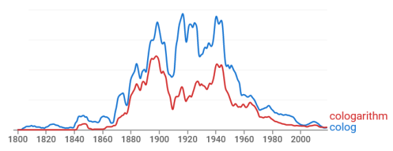
The cologarithm base b is the logarithm base 1/b, or equivalently, the negative of the logarithm base b.

cologb x = log1/b x = -logb x

I suppose people spoke of cologarithms more often when they did calculations with logarithm tables.

Entropy

There’s one place where I would be tempted to use the colog notation, and that’s when speaking of Shannon entropy.

The Shannon entropy of a random variable with N possible values, each with probability pi, is defined to be

-\sum_{i=1}^N p_i \log_b \, p_i

At first glace this looks wrong, as if entropy is negative. But you’re taking the logs of numbers less than 1, so the logs are negative, and the negative sign outside the sum makes everything positive.

If we write the same definition in terms of cologarithms, we have

 \sum_{i=1}^N p_i \,\text{colog}_b \, p_i

which looks better, except it contains the unfamiliar colog.

Bits, nats, and dits

These days entropy is almost always measured in units of bits, i.e. using b = 2 in the definition above. This wasn’t always the case.

When logs are taken base e, the result is in units of nats. And when the logs are taken base 10, the result is in units of dits.

So binary logs give bits, natural logs give nats, and decimal logs give dits.

Bits are sometimes called “shannons” and dits were sometimes called “bans” or “hartleys.” The codebreakers at Bletchley Park during WWII used bans.

The unit “hartley” is named after Ralph Hartley. Hartley published a paper in 1928 defining what we now call Shannon entropy using logarithms base 10. Shannon cites Hartley in the opening paragraph of his famous paper A Mathematical Theory of Communication.

Related posts

Corollary of a well-known fact

When students learn about decimals, they’re told that every fraction either has a terminating decimal expansion or a repeating decimal expansion. The previous post gives a constructive proof of the converse: given a repeating fraction (in any base) it shows how to find what rational number it corresponds to.

Maybe you learned this so long ago that it seems obvious. But here’s a corollary that I don’t believe is so obvious.

For any positive integer n and for any integer b > 1, with n and b relatively prime, there is some number of the form bk – 1 which is divisible by n.

So if I take some number, say 37, I can find a hexadecimal number consisting entirely of Fs which is divisible by 37. In fact FFFFFFFFF will do the trick. This is just the statement above with b = 16.

How does this follow from every rational number having a repeating decimal expansion?

Write 1/n as a repeating decimal in base b. (The assumption that n and b are relatively prime implies that the decimal repeats.) If the period of this decimal is k, then the previous post shows that 1/n is a multiple of 1/(bk – 1). It follows that n is a divisor of bk – 1.

Related post: A bevy of ones

Repeating decimals in any base

My previous post ended with a discussion of repeating binary decimals such as

0.00110011…two = 1/5.

For this post I’ll explain how calculations like that are done, how to convert a repeating decimal in any base to a fraction.

First of all, we only need to consider repeating decimals of the form

0.1b, 0.01b, 0.001b, etc.

because every repeating decimal is an integer times an expression like one above. For example,

0.424242… = 42 × 0.010101…

You can think of that example as base 10, but it’s equally true in any base that has a 4, i.e. any base greater than 4.

Now suppose we have an expression

0.\underbrace{000\ldots1}_{n \text{ terms}}\underbrace{000\ldots1}_{n \text{ terms}}\cdots

in base b.

We can see that this expressions is

\sum_{k=1}^\infty \left(b^{-n} \right )^k = \frac{1}{b^n - 1}

by summing a geometric series.

So going back to our example above,

0.010101\ldots_b = \frac{1}{b^2 -1}

If we’re working in base 10, this equals 1/99. If we’re working in hexadecimal, this is 1/FFhex = 1/255.

I’ll finish with a duodecimal example. Suppose we have

0.7AB7AB7AB…twelve

and want to convert it to a fraction. We have

0.7\text{AB}7\text{AB}\ldots_{\text{twelve}} = 7\text{AB}_{\text{twelve}} \times 0.001001\ldots_{\text{twelve}} = \frac{7\text{AB}_{\text{twelve}}}{BBB_{\text{twelve}}}

Or 1139/1727 in base 10.

Chaotic image out of regular slices

Yesterday I wrote about the bits in powers of 3. That post had a low-resolution image, which has its advantages, but here’s a higher resolution image that also has its advantages.

bits of 3^n

The image looks chaotic. I say this in the colloquial sense, not in the technical sense as in period three implies chaos. I just mean that the image looks noisy.

And yet every vertical slice of this image is periodic! The last n bits of each row depend only on the last n bits of its predecessor, and there are only 2n possible last bits. Some pattern of last n bits must reappear eventually, and when it does, the pattern will repeat from that point on.

To make this easier to see, imagine rotating the image above counterclockwise by 90 degrees. The rows in the image below correspond to the columns in the image above. I’ll print both the bit values and an on/off visualization as in the previous couple posts.

bits and graphical representation

Here’s the code that produced the image.

for k in range(6):
    bits = [(3**i & 2**k) >> k for i in range(64)]
    for bit in bits:
        print(bit, end='')
    print()  
    for bit in bits:
        print(chr(0x2588) if bit else ' ', end='')
    print("\n")

The array bits contains the first 64 bits in column number k, numbering columns from the right. That is, it contains the kth least significant bit of the first 64 powers of 3.

Now when I see a repeating pattern of digits, I think of decimal representations of rational numbers. If we put “0.” in front of the bit sequences above and think of them fractions, is there a pattern to these fractions?

In base two we have

    0.11111111... = 1
    0.01010101... = 1/3
    0.00000000... = 0
    0.00110011... = 1/5
    0.00011110... = 2/17

Can you detect a pattern in the rational numbers on the right side?

Evolution of random number generators

The previous post showed that the bits of prime powers look kinda chaotic. When you plot them, they form a triangular shape because the size of the numbers is growing. The numbers are growing geometrically, so their binary representations are growing linearly. Here’s the plot for powers of 5:

bits of powers of 5 plotted

You can crop the triangle so that you just see a rectangular portion of it, things look less regular. If we look at powers of p modulo a power of 2, say 232, then we’re chopping off the left side of the triangle.

Suppose we don’t start with 1, but start with some other number, call it a seed, and multiply by 5 every time. Would we get a chaotic pattern? Yes, and we have just invented the congruential random number generator. These RNGs have the form

xn+1 = a xn mod m

The RNG we implicitly described above would have a = 5 and m = 232. This is not a good choice of a and m, but it’s on to something. We can use different values of multiplier and modulus to make a decent RNG.

The RANDU random number generator, commonly used in the 1960’s, used a = 65539 and m = 231. This turned out to have notoriously bad statistical properties. We can see this with a small modification of the code used to produce the plot above.

    def out(s):
        s = s.replace('1', chr(0x2588))
        s = s.replace('0', ' ')
        print(s)    

    a, m = 65539, 2**31
    x = 7
    for i in range(32):
        x = a * x % m
        s = format(x, '32b')
        out(s)

Here’s the plot.

plotting bits of RANDU random number generator

The pattern on the right side looks like a roll of film. This shows that the lowest order bits are very regular. You can also see that we need to start with a large seed: starting with 7 created the large triangular holes at the top of the image. There are other patterns in the image that are hard to describe, but you get the sense something is not right, especially when you compare this image to a better alternative.

A much better choice of parameters is multiplier a = 48271 and modulus m = 231 -1. These are the parameters in the MINSTD random number generator. Here’s a plot of its bits, also starting with seed 7.

plot of MINSTD bits

The MINSTD generator is much better than RANDU, and adequate for some applications, but far from state of the art. You could do better by using a much larger multiplier and a modulus on the order of  264 or 2128.

You could do even better by adding a permutation step to your congruential generator. That’s the idea behind the PCG (permuted congruential generator) family of random number generators. These generators pass all the standard statistical tests with flying colors.

There are many other approaches to random number generation, but this post shows one thread of historical development, how hypothetically someone could go from noticing that prime powers have chaotic bit patterns to inventing PCG.

Related posts

Powers of 3 in binary

I was thumbing through A New Kind of Science [1] and one of the examples that jumped out at me was looking at the bits in the binary representation of the powers of 3. I wanted to reproduce the image myself and here’s the result.

bits of powers of 3 plotted

Here a white square represents a 1 and a blue square a 0. There’s a white border on the right edge because all powers of 3 are odd, i.e. end in 1 when written in binary.

As with many of the images in Wolfram’s book, it’s somewhere between regular and chaotic.

I produced the image at the command line with the following Python code.

    from numpy import log2

    N = 60
    k = int(log2(3)*N)+1

    for i in range(N):
        s = format(3**i, str(k)+'b')
        s = s.replace('1', chr(0x2588))
        s = s.replace('0', ' ')
        print(s)

The code writes powers of three as binary strings of length k where k is calculated so the last number in the sequence will fit. It then replaces 1s with a solid block character and replaces 0s with a blank space. My terminal has a blue background and a white foreground, so 1s show up as white squares and 0s as blue.

The characters in my terminal are twice as high as they are wide, so I changed the aspect ratio after taking the screen shot so that the blocks come out more square.

Update: Other bases

What if we look at bases other than 3?

Here’s the revised code to let you specify any base b.

    from numpy import log2

    def out(s):
        s = s.replace('1', chr(0x2588))
        s = s.replace('0', ' ')
        print(s)    

    b = 5
    N = 50
    k = int(log2(b)*N)+1

    for i in range(N):
        s = format(b**i, str(k)+'b')
        out(s)

Here’s what powers of 5 look like:

bits of powers of 5 plotted

And here’s what powers of 7 look like:

bits of powers of 7 plotted

What if our base isn’t prime? It doesn’t make an obvious difference if the base is odd, but if it’s even we get a skewed image. Here’s the plot for p = 6.

bits of powers of 6 plotted

This is just the plot for powers of 3 with the nth row shifted left by n positions.

Related posts

[1] I’ve looked through the book before for fun, but this time I’m looking through it with a practical project in mind. I never thought that would happen.

Factors of orders of sporadic groups

I was curious about the orders of the sporadic groups, specifically their prime factors, so I made a bar graph to show how often each factor appears.

To back up a little bit, simple groups are to groups roughly what prime numbers are to integers. Finite simple groups have been fully classified, and they fall into several infinite families of groups, except for 26 misfits, the so-called sporadic groups. The largest of these is nicknamed The Monster and has surprising connections to various areas of math.

One thing that jumps out  is that the order of every sporadic group is divisible by 2, 3, and 5. (In fact they’re all divisible by 120, i.e. by 2³, 3, and 5.) Another is that all the primes between 2 and 71 appear somewhere, except 53 and 61 are missing.

I don’t know whether there’s any significance to these patterns. Maybe they’re a simple consequence of things that people who work in this area know. I’m just noodling around here.

The Python code that produced the plot is given below.

Related posts

from sympy import primefactors
from collections import Counter
import matplotlib.pyplot as plt

orders = [
    95040, 
    175560, 
    443520, 
    604800, 
    10200960, 
    17971200, 
    44352000, 
    50232960, 
    244823040, 
    898128000, 
    4030387200, 
    145926144000, 
    448345497600, 
    460815505920, 
    95766656000, 
    42305421312000, 
    64561751654400, 
    273030912000000, 
    51765179004000000, 
    90745943887872000, 
    4089470473293004800, 
    4157776806543360000, 
    86775571046077562880, 
    1255205709190661721292800, 
    4154781481226426191177580544000000, 
    808017424794512875886459904961710757005754368000000000
]

c = Counter()
for o in orders:
    for f in primefactors(o):
        c[f] += 1

factors = sorted(c.keys())
frequencies = [c[k] for k in factors]

fig, ax = plt.subplots()
ax.bar([str(f) for f in factors], frequencies)
ax.set_xlabel("prime factor")
ax.set_ylabel("Number of groups")
ax.set_title("Prime factors of sporadic group orders")

Excessive, deficient, and perfect numbers

I learned recently that weekly excess deaths in the US have dipped into negative territory [1], and wondered whether we should start speaking of deficient deaths by analogy with excessive and deficient numbers.

The ancient Greeks defined a number n to be excessive, deficient, or perfect according to whether the sum of the number’s proper divisors was greater than, less than, or equal to n. “Proper” divisor means that n itself isn’t included. Excessive numbers are also called “abundant” numbers.

For example, 12 is excessive because

1 + 2 + 3 + 4 + 6 = 16 > 12,

8 is deficient because

1 + 2 + 4 < = 7 < 8,

and 6 is perfect because

1 + 2 + 3 = 6.

Perfect numbers

Nearly all numbers are excessive or deficient; perfect numbers constitute a very thin middle ground [2]. There are 51 known perfect numbers, all even so far. Euclid proved that if M is a Mersenne prime, then n = M(M+1)/2 is even and perfect. Euler proved the converse: if n is an even perfect number, n = M(M + 1)/2 for some Mersenne prime M.

No one has proved that odd perfect numbers don’t exist, but mathematicians keep proving more and more properties that an odd perfect number must have, if such a number exists. Maybe some day this list will include an impossibility, proving that there are no odd perfect numbers. Currently we know that if an odd perfect number exists, it must have more 1500 digits, its largest prime factor must have more than 8 digits, etc.

Density of excessive numbers

A little less than 1 in 4 numbers are excessive. More precisely, the proportion of excessive numbers less than N approaches a limiting value as N goes to infinity, and that limit is known to be between 0.2474 and 0.2480. See [3]. This means that a little more than 1 in 4 numbers is deficient.

Perfect number density

I said that perfect numbers form a thin middle ground between excessive and deficient numbers. We only know of 51 perfect numbers, but there may be infinitely many of them. Even so, they are thinly distributed, with zero density in the limit. So the density of deficient numbers is 1 minus the density of excessive numbers.

There is a conjecture that there are infinitely many perfect numbers, but that they are extremely rare. As stated above, n is a perfect prime if and only if n = M(M+1)/2 for a Mersenne prime M. A Mersenne prime is a prime number of the form 2p – 1 where p is prime. The number of such exponents p less than a given bound x is conjectured to be asymptotically proportional to

eγ log x / log 2

and the following graph gives empirical support for the conjecture. More on this conjecture here.

Predicted vs actual Mersenne primes

If the p‘s are thinly spread out, then the Mersenne primes, 2 raised to the power of these p‘s, are much more thinly spread out, and so even perfect numbers are very thinly spread out.

Related posts

[1] Based on CDC data

[2] Some sources define a number n to be excessive if the sum of its proper divisors is greater than or equal to n, meaning that by this definition perfect numbers are included in excessive numbers.

[3] Marc Deléglise Bounds for the density of abundant numbers

Is fast grep faster?

The grep utility searches text files for regular expressions, but it can search for ordinary strings since these strings are a special case of regular expressions. However, if your regular expressions are in fact simply text strings, fgrep may be much faster than grep. Or so I’ve heard. I did some benchmarks to see.

Strictly speaking I used grep -F rather than fgrep. On Linux, if you ask for the man (manual) page for fgrep you’ll be taken to the man page for grep which says

In addition, the variant programs egrep, fgrep and rgrep are the same as grep -E, grep -F, and grep -r, respectively. These variants are deprecated, but are provided for backward compatibility.

I was working on a project for a client where I had to search for a long list of words in a long list of files [1]. This is the kind of task where fgrep (“fast grep”) is supposed to be much faster than grep. It was a tiny bit faster, not enough to notice. When I timed it the difference was on the order of 1%.

I ran an analogous search on my own computer with different data and got similar results [2]. There may be instances where fgrep is much faster than grep, but I haven’t seen one first hand.

I suspect that the performance difference between fgrep and grep used to be larger, but the latter has gotten more efficient. Now grep is smart enough to search for strings quickly without having to be told explicitly via -F that the regular expressions are in fact strings. Maybe it scans the regular expression(s) before searching and effectively sets the -F flag itself if appropriate.

Related posts

[1] I used the -f to tell grep the name of a file containing the terms to search for, not to be confused with the additional flag -F to tell grep that the search terms are simply strings.

[2] I got similar results when I was using Linux (WSL) on my computer. When I used grep from GOW the -F flag made the search 24 times faster. Because the GOW project provides light-weight ports of Gnu tools to Windows, it’s understandable that it would not include some of the optimizations in Gnu’s implementation of grep.

Tower of powers and convergence

This post will look at the “tower of powers”

x^{x^{x^{\iddots}}}

and ask what it means, when it converges, and how to compute it. Along the way I’ll tie in two recent posts, including one that should come as a surprise.

First of all, the expression is right-associative. That is, it is the limit of

x^(x^(x^…))

and not the limit of

((x^x)^x)^…)

This means we evaluate our tower from the top down, which is a little strange to think about. But if we interpreted our tower as left-associative, building the tower from the bottom up, the sequence would be much less interesting: the limit would be 1 for 0 < x ≤ 1, and infinity for x > 1.

A few weeks ago I wrote about the special case of x equal to the imaginary unit. I looked at the sequence

i, i^i, i^{i^i}, \ldots

and the pattern the it makes in the complex plane.

We can see that the iterates converge to somewhere around 0.4 + 0.4i.

This post will replace i with a real number x. Leonard Euler discovered a long time ago that the “tower of power” converges for x between ee and e1/e. See[1].

Furthermore, for those x‘s where the sequence converges, it converges to an expression involving the Lambert W function which I wrote about in my previous post.

The power tower can be written in Donald Knuth’s up arrow notation as the limit of

x \uparrow \uparrow n

as n goes to infinity. The equation relating this limit to Lambert’s W function is

\lim_{n\to\infty}x\uparrow \uparrow n = - \frac{W(-\log x)}{\log x}

Let’s try this out numerically. Euler tells us the limit exists for x in the interval [eee1/e] which is roughly [0.07, 1.44].

We’ll do this at the Python REPL. First we import functions to compute log and W.

    >>> from math import log
    >>> from scipy.special import lambertw as w

Now if we have correctly found our limit y, then xy should equal y. The following shows that this is the case.

    >>> x = 0.07
    >>> y = -w(-log(x))/log(x)
    >>> y
    0.37192832251839264
    >>> x**y
    0.37192832251839264

    >>> x = 1.44
    >>> y = -w(-log(x))/log(x)
    >>> y
    2.3938117482029475
    >>> x**y
    2.393811748202947

By the way, we’ve said which real values of x cause the series to converge. But my first post on iterated powers looked at x = i. For which complex values does the series converge? I suspect the domain is a complicated fractal, but I don’t know that for sure.

Related posts

[1] Brian Hayes. Why W? American Scientist. Vol 93, pp 104–109.