First time seeing a rare event

Suppose you’ve been monitoring a rare event for a long time, then you see your first occurrence on the Nth observation. Now what would you say about the event’s probability?

For example, suppose you’re wondering whether dogs ever have two tails. You observe thousands of dogs and never see two tails. But then you see a dog with two tails? Now what can you say about the probability of dogs having two tails? It’s certainly not zero.

We’ll first look at the case of 0 successes out of N trials then look at the case of 1 success out of N trials.

Zero successes

If you’re observing a binary event and you’ve seen no successes out of N trials your point estimate of the probability of your event is 0. You can’t have any confidence in the relative accuracy of your estimate: if the true probability is positive, no matter how small, then the relative error in your estimate is infinite.

But you can have a great deal of confidence in its absolute accuracy. When you’re looking for a binary event and you have not seen any instances in N trials for large N, then a 95% confidence interval for the event’s probability is approximately [0, 3/N]. This is the statistical rule of three. This is a robust estimate, one you could derive from either a frequentist or Bayesian perspective.

Note that the confidence interval [0, 3/N] is exceptionally narrow. When observing a moderate mix of successes and failures the width of the confidence interval is on the order of 1/√N, not 1/N.

First success

After seeing your first success, your point estimate jumps from 0 to 1/N, and infinite relative increase. What happens to your confidence interval?

If we use Jeffreys’ beta(1/2, 1/2) prior, then the posterior distribution after seeing 1 success and N − 1 failures is a beta(3/2, N − 1/2). Now an approximate 95% confidence interval is

[0.1/N, 4.7/N]

So compared to the case of seeing zero successes, seeing one success makes our confidence interval about 50% wider and shifts it to the left by 0.1/N.

So if you’ve seen 100,000 dogs and only 1 had two tails, you could estimate that a 95% confidence interval for the probability of a dog having two tails is

[10−6, 4.7 × 10⁻⁵].

If we run the exact numbers we get

[ 1.07 × 10⁻⁶, 4.67 ×10⁻⁵].

Related posts

Stellar magnitude

Imagine the following dialog.

“Logarithms are usually taken to integer bases, like 2 or 10.”

“What about e?”

“OK, that’s an example of an irrational base, but it’s the only one.”

“Decibels are logarithms to base 101/10.”

“Really?!”

“Yeah, you can read about this here.”

“That’s weird. But logarithms are always take to bases bigger than 1.”

“Au contraire. Bases can be less than one, not just in theory but in practice.”

This post expands on the dialog above, especially the last line. We will show that stellar magnitude is a logarithm to a base smaller than 1.

Decibles are defined as 10 times the log base 10. But as explained here, decibels are not just a multiple of a logarithm, they are logarithms, logarithms base 101/10.

Irrational bases

Raising a musical pitch a half-step (semitone) multiplies its frequency by 21/12, and so raising it 12 half-steps doubles it, raising it an octave. Semitones are logarithms base 21/12.

So here are two examples of irrational bases for logarithms: decibels are logs base 1.2589 and semitones are logs base 1.0595.

Stellar magnitude

Vega

Stellar magnitude is strange for a couple reasons. First of all, the scale runs backward to what you might expect, with brighter objects having smaller magnitude. Perhaps stellar magnitude should be called stellar dimness. But the magnitude scale made more sense when it was limited to visible stars. The most visible starts were of the first category, the next most in the second category, and the least visible in the sixth category.

Second, stellar magnitude is defined so that a change in brightness of 100 corresponds to change in magnitude of 5. This seems arbitrary until you realize the intention was to fit a scale from 1 to 100 to the magnitude of visible stars. The scale seems strange now that we apply it to a wider variety of objects than naked eye astronomy.

If a star X is 100 times as bright as a star Y, then the magnitude of X is −5 times the magnitude of Y. The log base 10 of the brightness of X is twice the log base 10 of the magnitude of Y, so magnitude is −5/2 times log base 10 of brightness.

So stellar magnitude is a multiple of log base 10, like decibels.

Now

loga(x) = logb(x) / logb(a)

for any bases a and b. If we let b = 10, this says that a multiple k of base 10 is the same as the log base a where log10(a) = 1/k, so

a = 101/k.

For decibels, k = 10, so a = 101/10 = 1.2589. For stellar magnitude, k = −5/2, so a = 10−2/5 = 0.3981.

That is, stellar magnitude is logarithm base 0.3981.

To be more precise, we need a reference point. The star Vega (image above) has magnitude 0, so the magnitude of a star is the logarithm base 0.003162 of the ratio of the star’s brightness to the brightness of Vega.

Related posts

Image of Vega by Stephen Rahn via Wikipedia.

Area codes

US telephone area codes are allocated somewhat randomly. There was a deliberate effort to keep geographical proximity from corresponding to numerical proximity, unlike zip codes. (More of zip code proximity here.) In particular, consecutive area codes should belong to different states. The thought was that this would reduce errors.

It’s still mostly the case that states do not have consecutive area codes. But there is one exception: Colorado contains area codes 719 and 720. California, Texas, and New York all have a pair of area codes that differ by 2. For example, Tyler has area code 430 and Midland has area code 432. The median minimum difference between area codes within a state is 19.

I don’t know why this is. Only about 400 of the possible 1000 area codes are assigned to a geographic region. (Some are reserved for non-geographic uses, like toll-free numbers.) There’s no need to assign consecutive area codes within a state when adding a new area code.

I wrote a little script to look up the location corresponding to an area code. This is something I have to do fairly often in order to tell what time zone a client is probably in.

I debated whether to write such a script because it’s trivial to search for such information. Typing “area code 510” into a search bar is no harder than typing areacode 510 on the command line, but the latter is less disruptive to my workflow. I don’t have to click on any sketchy websites filled with adds, I’m not tempted to go anywhere else while my browser is open, and the script works when my internet connection is down.

The script is trivial:

    #!/usr/bin/env python3
    import sys

    codes = {
        "202" : "District of Columbia",
        "203" : "Bridgeport, CT",
        "204" : "Manitoba", 
        ....
        "985" : "Houma, LA",
        "986" : "Idaho",
        "989" : "Saginaw, MI",
    }

    area = sys.argv[1]
    print(codes[area]) if area in codes else print("Unassigned")

If you’d like, you can grab the full script here.

Curvature at Cairo

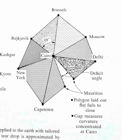
I was flipping through Gravitation [1] this weekend and was curious about an illustration on page 309. This post reproduces that graph.

The graph is centered at Cairo, Egypt and includes triangles whose side lengths are the distances between cities. The triangles are calculated using only distances, not by measuring angles per se.

The geometry of each triangle is Euclidean: giving the three edge lengths fixes all the features of the figure, including the indicated angle. … The triangles that belong to a given vertex [i.e. Cairo], laid out on a flat surface, fail to meet.

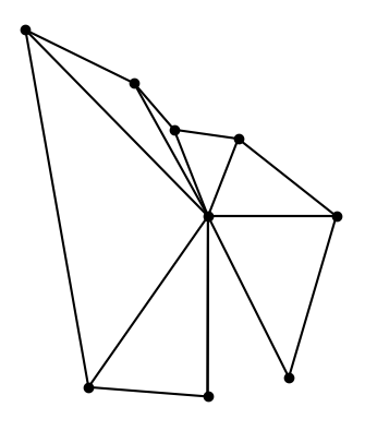
I will reproduce the plot in Python because I’m more familiar with making plots there. But I’ll get the geographic data out of Mathematica, because I know how to do that there.

Geographic information from Mathematica

I found the distances between the various cities using the GeoDistance function in Mathematica. The arguments to GeoDistance are “entities” which are a bit opaque. When using Mathematica interactively, you can use ctrl + = to enter the name of an entity. There’s some guesswork, e.g. whether I meant New York City or the state of New York when I entered “New York”, but Mathematica guessed correctly. The following code lists the city entities explicitly.

    cities = {
        Entity["City", {"Cairo", "Cairo", "Egypt"}], 
        Entity["City", {"Delhi", "Delhi", "India"}], 
        Entity["City", {"Moscow", "Moscow", "Russia"}], 
        Entity["City", {"Brussels", "Brussels", "Belgium"}], 
        Entity["City", {"Reykjavik", "Hofudhborgarsvaedhi", "Iceland"}], 
        Entity["City", {"NewYork", "NewYork", "UnitedStates"}], 
        Entity["City", {"CapeTown", "WesternCape", "SouthAfrica"}], 
        Entity["City", {"PortLouis", "PortLouis", "Mauritius"}] }

Most of these are predictable, but I would not have guessed the code for Reykjavik or Cape Town. I found these by using the command InputForm and entering the entities as above.

I found the distance from Cairo to each of the other cities with

    Table[GeoDistance[cities[[1]], cities[[i]]], {i, 2, 8}]

and the distances from the cities to their neighbors with

    Table[GeoDistance[cities[[i]], cities[[i + 1]]], {i, 2, 7}]
    GeoDistance[cities[[8]], cities[[2]]]

Drawing the plot

Now that we’ve got the data, how do we draw the plot?

Let’s put Cairo at the origin. First we draw a line from Cairo to Delhi. We might as well put Delhi on the x-axis to make things simple.

Next we need to plot Moscow. We know the distance R1 from Cairo to Moscow, and the distance R2 from Delhi to Moscow. So imagine drawing a circle of radius R1 centered at Cairo and a circle of radius R1 centered at Delhi. Moscow is located where the two circles intersect. The previous post shows how to find the intersection of circles.

The two circles intersect in at two points, so which do we choose? We choose the intersection point that preserves the orientation of the original graph (and the globe). As we go through the cities in counterclockwise order, the cross product of the previous line to the next line should have positive z component.

This shows that the original graph was not to scale, though the gap between triangles was approximately to scale. In hindsight this should have been obvious: Brussels and Reykjavik are much closer to each other than Capetown and New York are.

The gap

Why the gap? Because the earth is curved at Cairo (and everywhere else). If the earth were flat, the triangles would fit together without any gaps.

There’s no gap when you take spherical triangles on the globe. But even though the triangles preserve length when projected to the plane, they cannot preserve angles too. The sum of the angles in a spherical triangle adds up to more than 180°, and the amount by which the sum exceeds 180° is proportional to the size of the spherical triangle. Since the angles of triangles in the plane do add up to 180°, each flat triangle fails to capture a bit of the corresponding spherical triangles, and the failures add up to the gap we see in the image.

[1] Gravitation by Misner, Thorne, and Wheeler. 1973.

Calculating the intersection of two circles

Given the equations for two circles, how can you tell whether they intersect? And if they do intersect, how do you find the point(s) of intersection?

MathWorld gives a derivation, but I’d like to add the derivation there in two ways. First, I’d like to be more explicit about the number of solutions. Second, I’d like to make the solution more general.

The derivation begins with the simplifying assumption that one circle is centered at the origin and the other circle is centered somewhere along the x-axis. You can always change coordinates so that this is the case, and doing so simplifies the presentation. Undoing this simplification is implicitly left as an exercise to the reader. I will go through this exercise here because I want a solution I can use in software.

Finding the x coordinate

Suppose the first circle, the one centered at the origin, has radius R. The other circle is centered at (d, 0) for some d, and has radius r. The  x-coordinate of the intersection is shown to satisfy the following equation.

x = \frac{d^2 -r^2 + R^2}{2d}

When I got to this point in the derivation I was wondering what assumption was made that guaranteed there is a solution. Clearly if you increase d enough, moving the second circle to the right, the circles won’t intersect. And yet the derivation for x always succeeds, unless d = 0. If d does equal 0, the two circles are concentric. In that case they’re the same circle if R = r; otherwise they never intersect.

Finding the y coordinate

Why does the derivation for x always succeed even though the intersection might be empty? The resolution depends on the solution for y. What we’ve found is that if the circles intersect, the x coordinate of the point(s) of intersection is given by the equation above.

The y coordinate of the point(s) of intersection satisfies

 \begin{align*} y^2 &= \frac{4d^2R^2 - (d^2 - r^2 + R^2)^2}{4d^2} \\ &= \frac{(-d+r-R)(-d-r+R)(-d+r+R)(d+r+R)}{4d^2} \end{align*}

If the numerator is negative, there is no real solution, no intersection. If the numerator is zero, there is one solution, and the two circles are tangent. if the numerator is positive, there are two solutions.

The distance between the two intersection points, if there are two intersection points, is a = 2|y|. This will be needed below.

a = \frac{\sqrt{(-d+r-R)(-d-r+R)(-d+r+R)(d+r+R)}}{d}

General position

Now suppose we’re first circle is centered at (x0, y0) and the second circle is centered at (x1, y1). Again we let d be the distance between the centers of the circles. The circles intersect twice if d < R + r, once if d = R + r, and never if d > R + r.

Imagine for a moment shifting and rotating the plane so that (x0, y0) goes to the origin and goes to (d, 0). The length of the line segment between the two intersection points is still given by a above. And the distance from the center of the first circle to that line segment is given by the equation for x above.

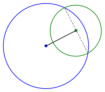
So to find the points of intersection, we first form a unit vector in the direction of the center of the first circle headed toward the center of the second circle. This is the black line at the top of the post. We move a distance x along this line, with x as in the equation above, and then move perpendicularly a distance a/2 in either direction. This is the dashed gray line.

Python code

The following code implements the algorithm described above.

    def circle_intersect(x0, y0, r0, x1, y1, r1):
        c0 = np.array([x0, y0])
        c1 = np.array([x1, y1])
        v = c1 - c0
        d = np.linalg.norm(v)
    
        if d > r0 + r1 or d == 0:
            return None
        
        u = v/np.linalg.norm(v)
        xvec = c0 + (d**2 - r1**2 + r0**2)*u/(2*d)
    
        uperp = np.array([u[1], -u[0]])
        a = ((-d+r1-r0)*(-d-r1+r0)*(-d+r1+r0)*(d+r1+r0))**0.5/d
        return (xvec + a*uperp/2, xvec - a*uperp/2)

Application

This post started out to be part of the next post, but it turned out to be big enough to make its own post. The next post looks carefully at an example that illustrates how you could discover that you’re living on a curved surface just by measuring the distances to points around you. I needed the code in this post to make the image in the next post.

A small programming language

Paul Graham said “Programming languages teach you not to want what they don’t provide.” He meant that as a negative: programmers using less expressive languages don’t know what they’re missing. But you could also take that as a positive: using a simple language can teach you that you don’t need features you thought you needed.

Awk

I read the original awk book recently, published in 1988. It’s a small book for a small language. The language has grown since 1988, especially the Gnu implementation gawk, and yet from the beginning the language had a useful set of features. Most of what has been added since then is of no use to me.

How I use awk

It has been years since I’ve written an awk program that is more than one line. If something would require more than one line of awk, I probably wouldn’t use awk. I’m not morally opposed to writing longer awk programs, but awk’s sweet spot is very short programs typed at the command line.

At one point when I was saying how I like little awk programs, someone suggested I use Perl one-liners instead because then I’d have access to Perl’s much richer set of features, in particular Perl regular expressions. Along those lines, see these notes on how to write Perl one-liners to mimic sed, grep, and awk.

But when I was reading the awk book I thought about how I rarely need the the features awk doesn’t have, not for the way I use awk. If I were writing a large program, not only would I want more features, I’d want a different language.

Now my response to the suggestion to use Perl one-liners would be that the simplicity of awk helps me focus by limiting my options. Awk is a jig. In Paul Graham’s terms, awk teaches me not to want what it doesn’t provide.

Regular expressions

At first I wished awk were more expressive is in its regular expression implementation. But awk’s minimal regex syntax is consistent with the aesthetic of the rest of the language. Awk has managed to maintain its elegant simplicity by resisting calls to add minor conveniences that would complicate the language. The maintainers are right not to add the regex features I miss.

Awk does not support, for example, \d for digits. You have to type [0-9] instead. In exchange for such minor inconveniences you get a simple but adequate regular expression implementation that you could learn quickly. See notes on awk’s regex features here.

The awk book describes regular expressions in four leisurely pages. Perl regular expressions are an order of magnitude more complex, but not an order of magnitude more useful.


Quadrature rules and an impossibility theorem

Many numerical integration formulas over a finite interval have the form

 \int_a^b f(x)\, dx = \sum_{i=1}^n w_i\, f(x_i) + C f^{(k)}(\xi)

That is, the integral on the left can be approximated by evaluating the integrand f at particular nodes and taking the weighted sum, and the error is some multiple of a derivative of f evaluated at a point in the interval [a, b].

This post will give several examples, showing how they all fit into to framework above, then discuss the impossibility of extending this framework to infinite integrals.

Simpson’s 3/8 rule

Simpson’s rule says

\int_{x_0}^{x_3} f(x) \, dx = \frac{3h}{8} \Big(f(x_0) + 3f(x_1) + 3f(x_2) + f(x_3) \Big)- \frac{3f^{(4)}(\xi) h^5}{80}

In this case the x‘s are evenly spaced a distance of h apart. The weights are 3h/8, 9h/8, 9h/8, and 3h/8.

We have n = 4, k = 4, and C = −3h5/80.

We don’t know a priori what the value of ξ will be, only that there will be some value of ξ between x0 and x3 that makes the equation hold. If we have an explicit bound on the 4th derivative of f then we have an explicit bound on the error in approximating the integral by the weighted sum.

Bode’s rules

A sequence of quadrature rules go by the name “Bode’s rule.” Here is one example, also known as Weddle’s rule.

\begin{align*} \int_{x_0}^{x_6} f(x)\, dx = \frac{h}{140}&\Big(41 f(x_0) + 216f(x_1) + 27 f(x_2) +272 f(x_3) \\ &+ 27 f(x_4) + 216 f(x_5) + 41 f(x_6) \Big) \\ &-\frac{9 f^{(8)}(\xi) h^9}{1400} \end{align}

As with Simpson’s 3/8 rule, you could map the formula for Bode’s rule(s) to the template at the top of the post.

Gauss quadrature

Gauss’ formula says

\int_{-1}^1 f(x)\, dx = \sum_{i=1}^n w_i\, f(x_i) + C f^{(2n)}(\xi)

for some ξ in [−1, 1]. Here the limits of integration are fixed, though you could use a change of variables to integrals over other finite integrals into this form.

Unlike Bode’s rule and Simpson’s rule, the x‘s are not evenly spaced but are the zeros of Pn, the Legendre polynomial of degree n. The weights are related to the x‘s and the derivative Pn evaluated at the x‘s. The constant C is a complicated function of n but is independent of f.

Note that the error term involves the (2n)th derivative of f. This explains why Gaussian integration can be more accurate than other methods using the same number of function evaluations. The non-uniform spacing of the integration nodes enables higher-order error terms.

Non-existence theorem

Although many integration rules over a finite interval have the form

 \int_a^b f(x)\, dx = \sum_{i=1}^n w_i\, f(x_i) + C f^{(k)}(\xi)

Davis and Rabinowitz [1] proved that there cannot be an integration rule of the form

\int_0^\infty f(x)\, dx = \sum_{i=1}^n w_i\, f(x_i) + C f^{(k)}(\xi)

The proof, given in [1], takes only about one page. The entire article is a little more than a page, and about half the article is preamble to the proof.

Related posts

[1] P. J. Davis and P. Rabinowitz. On the Nonexistence of Simplex Integration Rules for Infinite Integrals. Mathematics of Computation, Vol. 26, No. 119 (July, 1972), pp. 687–688

Jigs

In his book The World Beyond Your Head Matthew Crawford talks about jigs literally and metaphorically.

A jig in carpentry is something to hold parts in place, such as aligning boards that need to be cut to the same length. Crawford uses the term more generally to describe labor-saving (or more importantly, thought-saving) techniques in other professions, such as a chef setting out ingredients in the order in which they need to be added. He then applies the idea of jigs even more generally to cultural institutions.

Jigs reduce options. A craftsman voluntarily restricts choices, not out of necessity, but in order to focus attention where it matters more. Novices may chafe at jigs because they can work without them. Experts are even more capable of working without jigs than novices, but are also more likely to appreciate their use.

Style guides, whether in journalism or in software development, are jigs. They limit freedom of expression in minor details, ideally directing creativity into more productive channels.

Automation is great, but there’s a limit to how much we can automate our work. People often seek out a consulting firm precisely because there’s something non-standard about their project [1]. There’s more opportunity for jigs than automation, especially when delegating work. If I could completely automate a task, there would be no need to delegate it. Giving someone a jig along with a task increases the chances of the delegation being successful.

Related posts

[1] In my previous career, I sat through a presentation by a huge consulting company that promised to build software completely adapted to our unique needs, software which they had also built for numerous previous clients. This would be something they’ve never built before and something they have built many times before. I could imagine a more nuanced presentation that clarified what would be new and what would not be, but this presentation was blatantly contradictory and completely unaware of the contradiction.

Can the chi squared test detect fake primes?

Jeweler examining gemstones

This morning I wrote about Dan Piponi’s fake prime function. This evening I thought about it again and wondered whether the chi-squared test could tell the difference between the distribution of digits in real primes and fake primes.

If the distributions were obviously different, this would be apparent from looking at histograms. When distributions are more similar, visual inspection is not as reliable as a test like chi-squared. For small samples, we can be overly critical of plausible variations. For large samples, statistical tests can detect differences our eyes cannot.

When data fall into a number of buckets, with a moderate number of items expected to fall in each bucket, the chi squared test attempts to measure how the actual counts in each bucket compare to the expected counts.

This is a two-sided test. For example, suppose you expect 12% of items to fall in bucket A and 88% to fall in bucket B. Now suppose you test 1,000 items. It would be suspicious if only 50 items landed in bucket A since we’d expect around 120. On the other hand, getting exactly 120 items would be suspicious too. Getting exactly the expected number is unexpected!

Let’s look a the primes, genuine and fake, less than N = 200. We’ll take the distribution of digits in the list of primes as the expected values and compare to the distribution of the digits in the fake primes.

When I ran this experiment, I got a chi-squared value of 7.77. This is an unremarkable value for a sample from a chi-squared distribution with 9 degrees of freedom. (There are ten digits, but only nine degrees of freedom because if you rule out nine possibilities then digit is determined with certainty.)

The p-value in this case, the probability of seeing a value as large as the one we saw or larger, is 0.557.

Next I increased N to 1,000 and ran the experiment again. Now I got a chi-squared value of 19.08, with a corresponding p-value of 0.024. When I set N to 10,000 I got a chi-squared value of 18.19, with a corresponding p-value of 0.033.

When I used N = 100,000 I got a chi-squared value of 130.26, corresponding to a p-value of 10-23. Finally, when I used N = 1,000,000 I got a chi-squared value of 984.7 and a p-value of 3.4 × 10-206.

In short, the chi-squared test needs a fair amount of data to tell that fake primes are fake. The distribution of digits for samples of fake primes less than a thousand or so is plausibly the same as that of actual primes, as far as the test can distinguish. But the chi-squared values get implausibly large for fake primes up to  100,000.

Mastodon account

Mathstodon logo

I have an account on Mastodon: johndcook@mathstodon.xyz. Note that’s @math… and not @mast…

One advantage to Mastodon is that you can browse content there without logging, while Twitter is becoming more of a walled garden. You can browse my account, for example, by going to the URL

https://mathstodon.xyz/@johndcook

There’s hardly any content there at this time. I’m deciding what I want to use the account for.

Another advantage is that Mastodon, or at least the Mathstodon instance of Mastodon, supports LaTeX content via MathJax. This would be convenient if a thread has a few equations.

I’m certainly not going to create 18 accounts on Mastodon accounts like I did on Twitter. I’m thinking of maybe using my Mathstodon account to post highlights from my Twitter accounts, all in one account.

I’m concerned with where Twitter may be going. I do not plan to leave, though the site could change my mind.

I also have a Bluesky account, but I have no idea what if anything I’ll do with it. My handle there is johndcook@bsky.social.

One final note: You can subscribe to this blog by email or RSS here.

Update: I found out later that Mastodon accounts have associated RSS feeds, so mine is mathstodon.xyz/@johndcook.rss.