Fake primes

Someone asked on Math Overflow about the distribution of digits in primes. It seems 0 is the least common digit and 1 the most common digit.

Dan Piponi replies “this is probably just a combination of general properties of sets of numbers with a density similar to the primes and the fact that primes end in 1, 3, 7 or 9” and supports this by showing that “fake primes” have very similar digit distributions as actual primes. He generates the nth fake prime by starting with n log n and generating a nearby random integer ending in 1, 3, 7, or 9.

It seems like this fake prime function could be useful for studying more questions. Here is Dan Piponi’s Mathematica implementation:

    fakePrime[n_] :=
      With[
      {m = n Log[n]},
      10 RandomInteger[{Floor[0.09 m], Floor[0.11 m]}] + 
         RandomChoice[{1, 3, 7, 9}]
    ]

Do 5% less

I’ve been thinking about things that were ruined by doing about 5% more than was necessary, like an actor whose plastic surgery looks plastic.

Sometimes excellence requires pushing ourselves to do more than we want to do or more than we think we can do. But sometimes excellence requires restraint. Context is everything.

A few times the extra effort I’ve put into a report backfired. An illustration added to make things clearer caused confusion. (Or maybe it revealed confusion.)

I’ve made software harder to write and harder to use by having it do a little more than it should have, such as trying to fully automate something that should be 95% automated.

In the course of writing this post I’ve thought of several ways to expand it. I’ve drafted and deleted several versions of this concluding paragraph. But I’ll take my own advice and stop.

Tracking and the Euler rotation theorem

Suppose you are in an air traffic control tower observing a plane moving in a straight line and you want to rotate your frame of reference to align with the plane. In the new frame the plane is moving along a coordinate axis with no component of motion in the other directions.

You could do this in two steps. First, imagine the line formed by projecting the plane’s flight path onto the ground, as if the sun were directly overhead and you were watching the shadow of the plane move. The angle that this line makes with due north is the plane’s heading. You turn your head so that you’re looking horizontally along the projection of the plane’s path. Next, you look up so that you’re looking at the plane. The angle you lift your head is the elevation angle.

You’ve transformed your frame of reference by composing two rotations. Turning your head is a rotation about the vertical z-axis. Lifting your head is a rotation about the y-axis, if you label the plane’s heading the x-axis.

By Euler’s rotation theorem, the composition of two rotations can be expressed as a single rotation about an axis known as the Euler axis, often denoted e. How could you find the Euler axis and the angle of rotation about this axis that describes your change of coordinates?

You can find this calculation worked out in [1]. If the heading angle is α and the elevation angle is β then the Euler axis is

\mathbf{e} = \left( -\sin\frac{\alpha}{2} \sin \frac{\beta}{2},\,\, \cos \frac{\alpha}{2} \sin \frac{\beta}{2},\,\, \sin\frac{\alpha}{2} \cos\frac{\beta}{2} \right)

and the angle ϕ of rotation about e is given by

\phi = \arccos\left(\frac{\cos\alpha\cos\beta + \cos\alpha + \cos\beta - 1}{2}\right)

Related posts

[1] Jack B. Kuipers. Quaternions and Rotation Sequences. Princeton University Press. If I remember correctly, earlier editions of this book had a fair number of errors, but I believe these have been corrected in the paperback edition from 2002.

Using WordNet to create a PAO system

NLP software infers parts of speech by context. For example, the SpaCy NLP software can determine the parts of speech in the poem Jabberwocky even though the words are nonsense. More on this here.

If you want to tell the parts of speech for isolated words, maybe software like SpaCy isn’t the right tool. You might use lists of nouns, verbs, etc. This is what I’ll do in this post using the WordNet corpus. I’d like to show how you could use WordNet to create a mnemonic system.

PAO (person-action-object)

One way that people memorize six-digit numbers, or memorize longer numbers six digits at a time, is the PAO (person-action-object) system. They memorize a list of 100 people, 100 actions, and 100 direct objects. The first two digits of a six-digit number are encoded as a person, the next two digits as an action, and the last two digits as an object. For example, “Einstein dances with a broom” might encode 201294 if 20 is associated with Einstein, 12 with dance, and 94 with broom.

These mappings could be completely arbitrary, but you could memorize them faster if there were some patterns to the mappings, such as using the Major mnemonic system.

I’ve written before about how to use the CMU Pronouncing Dictionary to create a list of words along with the numbers they correspond to in the Major system. This post will show how to pull out the nouns and verbs from this list. The nouns are potential objects and the verbs are potential actions. I may deal with persons in another post.

Noun and verb lists in WordNet

The WordNet data contains a file index.noun with nouns and other information. We want to discard the first 29 lines of preamble and extract the nouns in the first column of the file. We can do this with the following one-liner.

   tail -n +30 index.noun | cut -d' ' -f1 > nouns.txt

Likewise we can extract a list of verbs with the following

   tail -n +30 index.verb | cut -d' ' -f1 > verbs.txt

There is some overlap between the two lists since some words can be nouns or verbs depending on context. For example, running

   grep '^read$' nouns.txt

and

   grep '^read$' verbs.txt

shows that “read” is in both lists. (The regex above anchors the beginning of the match with ^ and the end with $ so we don’t get unwanted matches like “treadmill” and “readjust.”)

Sorting CMU dictionary by part of speech

The following Python code will parse the file cmu_major.txt from here to pull out a list of nouns and a list of verbs, along with their Major system encodings.

    with open("nouns.txt") as f:
        nouns = set()
        for line in f.readlines():
            nouns.add(line.strip())
    
    with open("verbs.txt") as f:
        verbs = set()
        for line in f.readlines():
            verbs.add(line.strip())
    
    cmunouns = open("cmu_nouns.txt", "w")
    cmuverbs = open("cmu_verbs.txt", "w")
    
    with open("cmu_major.txt") as f:
        for line in f.readlines():
            w = line.split()[0].lower()
            if w in nouns:
                cmunouns.write(line)
            if w in verbs:
                cmuverbs.write(line)

You can download the output if you’d like: cmu_nouns.txt, cmu_verbs.txt.

Going back to the example of 201294, the file cmu_verbs.txt contains 82 words that correspond to numbers starting with 12. And the file cmu_nouns.txt contains 1,057 words that correspond to numbers starting with 94.

Choosing verbs is the hard part. Although there are verbs for every number 00 through 99, many of these would not be good choices. You want active verbs that can be combined with any subject and object.

My impression is that most people who use the PAO system—I do not—pick their names, verbs, and objects without regard to the Major system, and I could understand why: your choices are sometimes limited if you want to be compatible with the Major system. You might compromise and use Major-compatible pegs when possible and make exceptions as needed.

Memorizing four-digit numbers

The Major mnemonic system is a method of converting numbers to words that can be more easily memorized. The basics of the system can be written on an index card, but there are practical details that are seldom written down.

Presentations of the Major system can be misleading, intentionally or unintentionally, by implying that it is easy to find single words that encode numbers with three or four digits. Books and articles can unintentionally leave a wrong impression by being brief, but I can think of one book that I thought was intentionally misleading, opening with an example that was obviously reverse-engineered from its mnemonic. It was something like “Isn’t it easier to remember ‘constitution’ than 7201162?” Indeed it is, but I make up that example by starting with “constitution,” not starting with 7201162.

The Major system maps digits to consonant sounds. Spelling doesn’t matter, only pronunciation, and you can insert any vowels (or semivowels) you like. I list the mapping here in ARPAbet notation and here in IPA notation. The former is less precise but easier for most people to understand, so I’ll repeat it here.

0: S or Z
1: D, DH, T, or DH
2: N or NG
3: M
4: R
5: L
6: CH, JH, SH, or ZH
7: G or K
8: F or V
9: P or B

It is easy to find words that encode single digits. It’s a little harder to find words that encode some two-digit numbers, but it’s certainly doable. But if you want to encode all three-digit numbers as single words, you have to make some compromises. I estimate there’s about a 52% chance of being able to encode a four-digit number as a single word, for reasons I’ll explain below.

The CMU Pronouncing Dictionary lists 134,373 words along with their ARPAbet pronunciation. In this post I describe how I mapped the words to numbers, creating a file cmu_major.txt.

Not every three-digit number is in this file. The command

    grep -P -o ' \d{3}$' cmu_major.txt | sort -u | wc -l

shows that there are 958 unique three-digit numbers in the file, i.e. 42 three-digit numbers cannot be encoded as words in the CMU dictionary. By changing the ‘3’ to a ‘4’ in the one-liner above we see there are 5,191 unique four-digit numbers in the file, i.e. about 52% of all possible four-digit numbers.

Since it is very often not possible to encode numbers with four or more digits as single words, a common approach is to not try. Instead, just pay attention to the first three digits that a word would encode. The advantage of this is that it opens up more possibilities for encoding three-digit numbers. The downside is that you give up the possibility of encoding four-digit numbers in a single word, but this isn’t giving up much since there’s a 40% chance you’d fail anyway.

So if you want to memorize a four-digit number, you could memorize a pair of two-digit numbers. Some people like to draw these two numbers from different sets, such as using the name of a person for the first two digits and an action for the second two digits. I’ll explore this more in my next post on the PAO system.

The numerical range ellipse

Let A be an n × n complex matrix. The numerical range of A is the image of x*Ax over the unit sphere. That is, the numerical range of A is the set W(A) in defined by

W(A) = {x*Ax | x ∈ ℂn and ||x|| = 1}

where x* is the conjugate transpose of the column vector x.

The product of a row vector and a column vector is a scalar, so W(A) is a subset of the complex plane ℂ.

When A is a 2 × 2 matrix, W(A) is an ellipse, and the two foci are the eigenvalues of A.

Denote the two eigenvalues by λ1 and λ2 . Denote the major and minor axes of the ellipse by a and b respectively. Then

b² = tr(A*A) − |λ1|² − |λ2|².

where tr is the trace operator. This is the elliptical range theorem [1]. The theorem doesn’t state the major axis a explicitly, but it can be found from the two foci and the minor axis b.

Demonstration

We will create a visualization the numerical range of a matrix directly from the definition, generating x‘s at random and plotting x*Ax. Then we draw the ellipse described in the elliptical range theorem and see that it forms the boundary of the random points.

The following code plots 500 random points in the numerical range of a matrix formed from the numbers in today’s date. The eigenvalues are plotted in black.

import numpy as np
from scipy.stats import norm
import matplotlib.pyplot as plt

A = np.array([[8, 16], [20, 23j]])

for _ in range(5000):
    v = norm(0, 1).rvs(size=4)
    v /= np.linalg.norm(v)
    x = np.array([v[0] + 1j*v[1], v[2] + 1j*v[3]])
    z = np.conj(x).dot(A.dot(x))
    plt.plot(z.real, z.imag, 'o', color='0.9')

eigenvalues, eigenvectors = np.linalg.eig(A)    
plt.plot(eigenvalues[0].real, eigenvalues[0].imag, 'ko')
plt.plot(eigenvalues[1].real, eigenvalues[1].imag, 'ko')

The following code draws the ellipse guaranteed by the elliptical range theorem.

A_star_A = np.dot(np.conj(A).T, A)
b = (np.trace(A_star_A) - abs(eigenvalues[0])**2 - abs(eigenvalues[1])**2)**0.5
c = 0.5*abs(eigenvalues[0] - eigenvalues[1])
a = (2/3)*(2*(2*b**2/4 + c**2)**0.5 + c)

t = np.linspace(0, np.pi*2)
z = a*np.cos(t)/2 + 1j*b*np.sin(t)/2
u = (eigenvalues[1] - eigenvalues[0])/2
u /= np.linalg.norm(u)
m = eigenvalues.mean()
z = z*u + m

plt.plot(z.real, z.imag, 'b-')

Here is the result.

Here is the result of running the same code with 10,000 random points.

Related posts

[1] Ulrich Daepp, Pamela Gorkin, Andrew Shaffer, and Karl Voss. Finding Ellipses: What Blaschke Products, Poncelet’s Theorem, and the Numerical Range Know about Each Other. MAA Press 2018.

Random slices of a sphube

Ben Grimmer posted something yesterday on Twitter:

A nice mathematical puzzle🧐

If you take a 4-norm ball and cut it carefully, you will find a two-norm ball. 3D printed visual evidence below.
The puzzle: Why does this happen and how much more generally does it happen?

(This question was first posed to me by Pablo Parrilo)

This is a surprising result, and it touches on two things I’ve written about before.

Several years ago I wrote about the surprising result that if you slice open a Menger sponge a certain way then you can see six-pointed stars. I was just as surprised to see the result above. I also wrote several posts about “squircles,” and the 4-norm ball is a 3D version of the squircle, sometimes called a “sphube.”

I modified the code I’d written for the Menger sponge post to create random slides of the 4-norm ball. Here are some of the results.

One of these happens to be a circle, or at least close enough that it looks like a circle.

My code generated a random point and a random normal vector to determine a plane through that point. That’s how I produced the square-ish and triangle-ish plots.

For the last image, I set the normal vector to (1, 1, 1) because the 3D printed image above suggested that would be the right direction. I generated random points inside the cube, and one time the random point was approximately (0.2, 0, -0.2) and noticed the plot was approximately circular. It seems that when z = −x and the normal vector is (1, 1, 1) you get a circular cross section. By symmetry you can make many more examples from this example.

I have not proved anything yet; just played with plots.

Twin stars and twin primes

Are there more twin stars or twin primes?

If the twin prime conjecture is true, there are an infinite number of twin primes, and that would settle the question.

We don’t know whether there are infinitely many twin primes, and it’s a little challenging to find any results on how many twin primes we’re sure exist.

According to OEIS, we know there are 808,675,888,577,436 pairs of twin primes less than 1018.

There are perhaps 1024 stars in the observable universe. If so, there are certainly less than 1024 pairs of binary stars in the observable universe. In our galaxy about 2/3 of stars are isolated and about 1/3 come in pairs (or larger clusters). If that holds in every galaxy, then the number of binary stars is within an order of magnitude of the total number of stars.

Do we know for certain there are at least 1024 twin primes? It doesn’t seem anybody is interested in that question. There is more interest in finding larger and larger twin primes. The largest pair currently know have 388,342 digits.

The Hardy-Littlewood conjecture speculates that π2(x), the number of twin prime pairs less than x, is asymptotically equal to the following

\pi_2(x) \sim C_2 \int_2^x \frac{dt}{(\log t)^2}

where C2 is a constant, the product of (1 − 1/(p − 1)²) over all odd primes. Numerically C2 = 0.6601618….

When x = 1018 the right hand side of the Hardy Littlewood conjecture agrees with the actual number to at least six decimal places. If the integral gives an estimate of π2(x) within an order of magntude of being correct for x up to 1028, then there are more twin primes than twin stars.

It’s interesting that our knowledge of both twin stars and twin primes is empirical, though in different ways. We haven’t counted the number of stars in the universe or, as far as I know, the number of twin primes less than 1028, but we have evidence that gives us reason to believe estimates of both.

Simple way to distribute points on a sphere

Evenly placing points on a sphere is a difficult problem. It’s impossible in general, and so you distribute the points as evenly as you can. The results vary according to how you measure how evenly the points are spread.

However, there is a fast and simple way to distribute points that may be good enough, depending on your application, called the Fibonacci lattice.

Let P = 2N + 1. To distribute P points on a sphere let the latitude of the points be arccos(2i/P) and the longitude 2πi/φ where φ is the golden ratio and i runs from −N to N.

Here’s the Mathematica code that produced the image above.

    sp[{r_, lat_, long_}] := r {Cos[lat] Cos[long], Cos[lat] Sin[long], Sin[lat]};
    n = 500;
    Graphics3D@{ 
        Sphere[{0, 0, 0}, 1],
        Point[sp /@ 
            Table[{1, ArcSin[2 i /(2 n + 1)], 2 Pi i/GoldenRatio}, 
                  {i, -n, n}]]}

Maybe you’d like something that looks more random, i.e. something that looks what people think randomness looks like. Actual randomness is clumpier than people expect. In this case you could jitter the Fibonacci lattice by changing the coordinates to something like

    {1, ArcSin[2 i /(2 n + 1)] + RandomReal[0.05], 2 Pi i/GoldenRatio + RandomReal[0.1]}

Note that this adds twice as much randomness to the longitude than latitude because the former has twice the range.

Related posts

Spherical coordinate Rosetta Stone

If you’ve only seen one definition of spherical coordinates, you may be shocked to discover that there are multiple conventions. In particular, mathematicians and geoscientists have different conventions. As Volker Michel put it in book on constructive approximation,

Many mathematicians have faced weird jigsaw puzzles with misplaced continents after using a data set from a geoscientist.

Nor are there only two conventions. This post will cover three conventions, which I will call physics, math, and geography. This is not to imply that everyone in a profession uses the conventions named after the profession.

As with Fourier transforms there are many conventions. Presumably the reason for the proliferation of conventions is the same: a useful basic concept will be discovered multiple times in different areas of application. When there are trade-offs between conventions, people working in each area will choose the convention that is simplest for the things they care most about.

Questions and definitions

Given a triple of numbers (c1, c2, c3), that represent spherical coordinates, there are two basic questions:

  1. What do the numbers mean?
  2. What symbol should be used to represent them?

Part of the meaning question is whether the coordinate system is left-handed or right-handed. There is also a minor question of the standard range of equivalent angles.

Polar angle is the angle down from the positive z-axis, the north pole. The north pole has polar angle 0 and the south pole has polar angle π.

Latitude is the angle up from the xy plane or the equator. The latitude of the north pole is π/2 and the latitude of the south pole is −π/2.

Azimuth is the angle from an initial meridian (e.g. the Prime Meridian in geography). In mathematical terms it is the angle between the x-axis and a line connecting the projection of a point to the xy to the origin.

Physics convention

The physics convention is also the ISO 80000-2 convention. The three coordinates are

(radial distance to origin, polar angle, azimuthal angle)

and are conventionally denoted

(r, θ, ϕ).

The point (r, θ, ϕ) corresponds to

(r sin θ cos ϕ, r sin θ sin ϕ, r cos θ)

in Cartesian coordinates.

The coordinate system is right-handed: ϕ increases in the counterclockwise direction when looking down on the xy plane.

The polar angle typically runs from 0 to π and the azimuthal angle typically runs from 0 to 2π.

Math convention

In this convention the three coordinates are

(radial distance to origin, azimuthal angle, polar angle)

and are denoted

(ρ, θ, ϕ).

When compared to the physics notation we have something of a Greek letter paradox. Both conventions agree that the second coordinate should be written θ and the third coordinate should be written ϕ, but the two conventions mean opposite things by the two symbols.

The advantage of using θ to denote the azimuthal angle is that then θ has the same meaning as it has in polar coordinates. Similarly, the advantage of using ρ rather than r is to preserve the meaning of r in polar and cylindrical coordinates: ρ is the distance in 3 dimensions from a point to the origin, and r is the distance in 2 dimensions from the projection of a point to the xy plane and the origin.

Sometimes you’ll see r rather than ρ for the first coordinate.

The point (ρ, θ, ϕ) corresponds to

(ρ cos θ sin ϕ, ρ sin θ sin ϕ, ρ cos ϕ).

The math convention uses the same orientation and typical range coordinate ranges as the physics convention.

Geography and geoscience

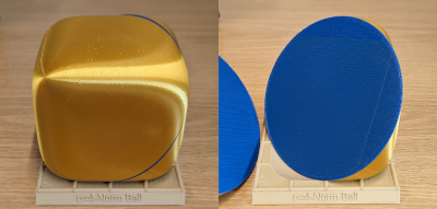
Geographic coordinate systems are complicated by the fact that the earth is not perfectly spherical. Geographic latitude and geocentric latitude are not exactly the same as the following highly exaggerated diagram shows.

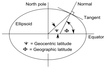
However, for this post we will assume a perfectly spherical earth in which geographic and geocentric latitudes are the same.

A point on the earth’s surface is described by two numbers, latitude and longitude. This corresponds to spherical coordinates in which the first coordinate is implicitly the earth’s radius. You’ll see latitude and longitude listed in either order.

The polar angle is sometimes called colatitude because latitude is the complementary angle of latitude. Longitude corresponds to azimuth. There are multiple symbols used for latitude, though λ is common for longitude. If you see one coordinate denoted λ, the other is latitude.

The safest, most explicit notation is to use the words longitude and latitude, not depending on symbols or order. Longitude is implicitly longitude east of the Prime Meridian, but to be absolutely clear, put an E at the end. Latitude typically ranges from −π/2 to π/2 (−90° to 90°). Longitude either runs from 0 to 2π or from −π to π (−180° to 180°).

To convert to Cartesian coordinates, set polar angle to π/2 − latitude, azimuth to longitude (east), and use the formulas above for either the physics or mathematics notation. If you have elevation, this is the radial distance above the earth’s surface, so ρ is the earth’s radius plus elevation.

Related posts